
Python Language
2. Python Statements, Objects, and Loops
2.1 Introduction to Objects and Classes
2.2 Built-in Data Types
2.3 Arithmetic Operators and Expressions
2.4 Variables and Assignment Statement
2.5 Python Objects and Their Memory Representation
2.6 Introduction to Looping
Objectives
- To introduce Python objects and classes, and the Python data types and operations on them.
- To introduce NumPy arrays and operations on them.
- To introduce basic Python statements that are most useful for working with TCAD Sentaurus tools.
- To understand how Python objects are stored in memory.
- To introduce looping in Python.
2.1 Introduction to Objects and Classes
The scripts discussed here are available in the directory
Applications_Library/GettingStarted/python/py_basics. The code examples
that must be entered at the interactive prompt are also available in this
Sentaurus Workbench project.
Click to view the primary file
python_pyt.py.
Everything is an object in Python. All data in Python programs is represented by objects. Numbers and strings are objects in Python. For example, the number 42 is an int object, and the number 3.141 is a float object. The string 'Hello, World!' is a str object. All data structures such as lists, tuples, and NumPy arrays are objects. Even Python functions, modules, and files are objects.
Everything in Python behaves as if it is an object created from some class. All built-in types such as numbers, strings, and lists are created from a class. In addition, you can create your own data types by defining a class. For example, in Section 3.3.2 User-Defined Classes, you will create a class to represent two-dimensional (2D) vectors.
Objects have a type and value. In Python, type and class are synonyms. In addition, since all values are represented by objects, for simplicity, the word value is often used instead of object. However, objects are more than values. They have attributes, which can be of two types: data attributes (variables defined inside a class) and methods (functions defined inside a class). Objects and classes are discussed in Section 3.3 Objects and Classes.
2.2 Built-in Data Types
Values in Python are of different types. A data type or simply type is a set of values and a set of operations that can be performed on those values. This section discusses Python data types. Arithmetic operations are discussed in Section 2.3 Arithmetic Operators and Expressions.
Python has several built-in data types that are always available. The built-in data types can be divided into primitive and compound data types.
Primitive data types are numeric types (such as integers, floating-point numbers, and complex numbers), Booleans, NoneType, and strings.
Compound data types (also called data structures) are used to group values. Some of these are lists, tuples, and dictionaries.
In addition to built-in data types, compound data types such as N-dimensional arrays and pandas DataFrame are available in the Python packages NumPy and pandas, respectively. These are useful for scientific computing.
2.2.1 Numeric Types: int, float, and complex
As discussed in The Python Standard Library, integers are created using numeric literals (a sequence of digits with or without a leading plus (+) or minus (-) sign):
>>> 3000  # create integer
3000
As with everything else in Python, numbers are represented by objects. You can find the class or type of a number using the built-in type function:
>>> type(3000)
<class 'int'>
The type or class of the value 3000 is int.
To create a floating-point number, include a decimal point:
>>> 3000.0  # create float using decimal point
3000.0
>>> type(3000.0)  # type of 3000.0 is float
<class 'float'>
You can also create floating-point numbers using scientific notation, which consists of a number (mantissa) followed by e, followed by an integer (exponent):
>>> 3.0e3  # Create float using scientific notation
3000.0
As defined by Sedgewick et al.: A literal is a Python-code representation of a data-type value. For example, both the literals 3000.0 and 3e3 represent the float value 3000.0:
>>> 3000.0
3000.0
>>> 3.0e3
3000.0
Python has built-in support for complex numbers. To create a purely imaginary number (a complex number with a zero real part), append j or J to a numeric literal. Unlike mathematical notation where i is used to denote the imaginary unit, Python uses j or J. The literals 1j and 1J represent the imaginary unit \( i = √{-1} \):
>>> 1j
1j
So, you can create the purely imaginary number \( 3 × 10^2 i \) as follows:
>>> 3e2j
300j
You can create a complex number by adding a purely imaginary number to a real number:
>>> 300 + 3e2j
(300+300j)
>>> type(3e2j)
<class 'complex'>
>>> type(300 + 3e2j)
<class 'complex'>
The type of both purely imaginary numbers and complex numbers is complex.
Both the literals 1j and 0 + 1j create a purely imaginary number:
>>> 0 + 1j
1j
To create complex numbers using expressions, you need to multiply by the imaginary unit 1j or 1J (see Section 3.1.3 Mathematical Constants for an example).
2.2.2 Boolean Type
The Boolean type stores logical information. There are only two values of Boolean type: True and False.
>>> False
False
>>> True
True
>>> type(True)  # type of True is bool
<class 'bool'>
2.2.3 NoneType
Python has a special value None, which is used to represent the absence of a value:
>>> None
In interactive mode, Python does not show any output after it evaluates None.
The type of the special value None is NoneType.
>>> type(None)
<class 'NoneType'>
You can explicitly print a None value:
>>> print(None)
None
For details about how to use None, see Section 3.2 Functions.
2.2.4 Built-in Constants
The special values True, False, and None are not strings. They are constants that are predefined in Python.
For a complete list of built-in constants, see The Python Standard Library: Built-in Constants.
2.2.5 Introduction to Sequence Types
Strings, lists, tuples, and 1D NumPy arrays are sequence-type data structures. A sequence is an ordered collection of values. A string is a sequence of characters.
Both lists and tuples can contain values of any type. They can contain primitive data types and compound data types. A list is a mutable data type; whereas, a tuple is an immutable data types. When a tuple is created, its contents cannot be changed, but you can change the contents of a list (see Section 2.5.5.1 Mutability of Objects).
2.2.5.1 Strings
As discussed in The Python Standard Library: Text Sequence Type — str, a Python string can be created in different ways. You can create a string by enclosing characters in either single quotation marks (') or double quotation marks ("):
>>> 'Hello, World'
'Hello, World'
>>> "Hello, World"
'Hello, World'
Strings are of type str:
>>> type('Hello, World')
<class 'str'>
As discussed in The Python Tutorial: Strings, \n is the newline character and the backslash (\) can be used to escape quotation marks in a string. You can use double quotation marks inside a string created using single quotation marks or single quotation marks inside a string created using double quotation marks. As a result, there is usually no need to use the backslash to escape quotation marks:
>>> "That\'s not what I said!"
"That's not what I said!"
>>> "That's not what I said!"
"That's not what I said!"
Strings can also be created using either three single quotation marks (''') or three double quotation marks ("""). Such triple-quoted strings can span multiple lines – all associated whitespace such as newlines are included in the string literal. For example:
>>> '''This is
... a multiline string
... '''
'This is\na multiline string\n'
The output produced by evaluating a string contains the enclosing quotation marks. The output produced by the print function is more readable since it does not contain the enclosing quotation marks. In addition, the newline character creates a newline in the output:
>>> print('''This is
... a multiline string
... '''
... )
This is
a multiline string
As shown in Section 1.3.1 Commenting Python Code, triple-quoted strings can be used to create block comments:
# Script: comment.py
# This script illustrates various comment types
# This is a single-line comment
"""
This is a multiline comment
x = 10
y = 20
w = x + y
print(w)
"""
x = 1  # This is an inline comment
y = 2
z = x + y
print(z)
> gpythonsh comment.py
3
Executing this script prints 3 instead of 30, which shows that Python does not execute parts of the code that are enclosed within triple-quoted strings.
As discussed in Section 3.2 Functions, triple-quoted strings are also used to create docstrings. Formatted string literals are another type of Python string, which are discussed in Section 2.4.3.1 Formatted Strings (f-Strings) and Format Specification.
2.2.5.2 Lists and Tuples
You can create a list by enclosing comma-separated values in brackets:
>>> [1, 2.4, True, None, 'Python']  # list object
[1, 2.4, True, None, 'Python']
You can create a tuple using comma-separated values, with or without parentheses:
>>> (1, 2.4, True, None, 'Python')  # creating tuple with parentheses
(1, 2.4, True, None, 'Python')
>>> 1, 2.4, True, None, 'Python'  # creating tuple without parentheses
(1, 2.4, True, None, 'Python')
A tuple is also created when you evaluate comma-separated expressions:
>>> 1 + 2, 1 * 2
(3, 2)
Expressions are discussed in Section 2.3 Arithmetic Operators and Expressions.
In general, lists and tuples can contain heterogeneous (different types of) values as can be seen from these examples. A list or tuple that contains values of the same type (for example, integers or floats) is known as a homogeneous list or tuple. For example:
>>> [1, 2, 3]  # all values are integers
[1, 2, 3]
>>> (1.0, 2.0, 3.0)  # all values are floats
(1.0, 2.0, 3.0)
2.2.5.3 One-Dimensional NumPy Arrays
You can create one-dimensional (1D) NumPy arrays by passing a homogeneous list or tuple to the array function in the NumPy package. Packages and functions are discussed in the following sections:
The NumPy package is not part of Python and must be imported using the import statement:
>>> import numpy as np # import NumPy package
Here, as np means Python will import the NumPy package and rename it to np for brevity. To use functions from the NumPy package such as the array function, you must now write np.array instead of numpy.array. For example:
>>> # Create 1D NumPy array using a list of integers
>>> np.array([1, 2, 3])
array([1, 2, 3])

>>> # Create 1D NumPy array using a tuple of floats
>>> np.array((1.0, 2.0, 3.0))
array([1., 2., 3.])
Expressions such as np.array contain a period (.). Therefore, this syntax for accessing functions is known as dot notation. Dot notation for modules is discussed in Section 3.1.2.1 Modules as Objects.
NumPy arrays are objects of type ndarray (N-dimensional array):
>>> type(np.array([1, 2, 3, 4]))
<class 'numpy.ndarray'>
The output numpy.ndarray shows the name of the class in dot notation. It indicates that the ndarray class is defined in the numpy package.
Python also supports arrays with the help of the array module. However, NumPy arrays are commonly used for scientific computing since they have the following advantages over the arrays and lists of Python:
- NumPy arrays are multidimensional.
- They are memory-efficient data structures.
- Computations using NumPy arrays are fast compared to computations using lists.
- They support vectorized operations (see
Section 3.1.4.2 Scalar-Oriented Versus Vectorized Code) through:
- Elementwise arithmetic operations (see Section 2.3.3 NumPy Array Operations)
- Vectorized mathematical functions called ufuncs (see Section 3.2.1.4 NumPy Universal Functions)
- They can be used to represent mathematical vectors (see Section 2.3.3 NumPy Array Operations) and matrices. Both NumPy and SciPy contain linear algebra functions for manipulating vectors and matrices.
Because of these advantages, NumPy arrays are used to store and process data by packages in the Python Scientific Computing Stack (see Section 3.1.1.3 Python Scientific Computing Stack) such as SciPy.
In this Tutorial, the term array always means a NumPy array.
2.2.5.4 Indexing Sequences
The values in a sequence are called items or elements. The number of elements in a sequence is called the length of the sequence, which you can find using the built-in len function:
>>> len([1, 2.4, True, None, 'Python'])
5
The number of elements in an array is known as the size of the array. You can find the size of a 1D array by using the len function:
>>> len(np.array([1, 2, 3, 4]))
4
Each element in a sequence is identified by an integer called its index. In Python, the index of a sequence is from 0 to length – 1.
You can access individual elements of a sequence using the index. This operation is known as indexing. To access a sequence element, you specify the name of the sequence and the element index inside brackets: sequence[index]
For example:
>>> [10, 20, 30, 40][0]  # first element or element in position 0
10
>>> [10, 20, 30, 40][1]  # second element or element in position 1
20
In Python, indices can be negative integers. Positive indices identify the position of the elements relative to the start of the sequence. Negative indices do so relative to the end of the sequence; instead of counting from the left, you start counting from the right. The index of the last element is -1, the index of the second-last element is -2, and so on:
>>> [10, 20, 30, 40][-1]  # last element
40
>>> [10, 20, 30, 40][-2]  # second-last element
30
Trying to access an element that does not exist or using an index that is not an integer results in an error:
>>> [10, 20, 30, 40][5]  # fifth element or element in position 4
Traceback (most recent call last):
  File "<stdin>", line 1, in <module>
IndexError: list index out of range

>>> [10, 20, 30, 40][4.1]
<stdin>:1: SyntaxWarning: list indices must be integers or slices, not float;
perhaps you missed a comma?
Traceback (most recent call last):
  File "<stdin>", line 1, in <module>
TypeError: list indices must be integers or slices, not float
Indexing a 1D NumPy array is similar to indexing lists:
>>> np.array([1, 2, 3, 4])[0]  # first element
1
>>> np.array([1, 2, 3, 4])[-1]  # last element
4
Section 4.3 More on Sequence Types discusses how to create some special sequences as well as additional operations on sequence types such as indexing. It also discusses list and string methods.
2.2.6 Introduction to Dictionaries
Python dictionaries are a collection of key–value pairs. The keys must be unique and can be any immutable type such as strings and numbers (see Section 2.5.5.1 Mutability of Objects). The keys can also be tuples if the tuple contains only strings, numbers, or tuples. The values can be of any type.
You can create a Python dictionary by enclosing a set of key–value pairs inside a pair of braces. Each key is associated with a value, and they are separated by a colon (:). For example, the following dictionary has two key–value pairs:
>>> {'x': 1, (1, 1): [10, 20]}
{'x': 1, (1, 1): [10, 20]}
The string 'x' and the tuple (1, 1) are the keys associated with the values 1 and [10, 20], respectively.
The type of a dictionary is dict:
>>> type({'x': 1, (1, 1): [10, 20]})
<class 'dict'>
Since each key is associated with a value, dictionaries are indexed by keys unlike sequences that are indexed by numbers (see Section 2.2.5.4 Indexing Sequences). Similar to sequences, you can use the key inside brackets to access the associated value. For example:
>>> # Use key 'x' to access value 1
>>> {'x': 1, (1, 1): [10, 20]}['x']
1
Unlike lists that are sequence types, Python dictionaries are mapping types (see The Python Standard Library: Mapping Types — dict). Python dictionaries are similar to Tcl arrays.
2.3 Arithmetic Operators and Expressions
In Python, operations on data are performed using operators, functions, and methods. Expressions are formed using a combination of literals, variable names, operators, function calls, and method calls.
You can use the interactive Python shell as a calculator. You can enter expressions or statements at the prompt and execute the code by pressing the Enter key. Python evaluates the expression and prints its value:
>>> 3 + 5  # Addition
8
>>> 0.5 ** 2 # Exponentiation
0.25
2.3.1 Scalar Operations
Single numbers are also called scalars. Operations between single numbers are scalar operations, and they result in another single number (scalar). The syntax for using binary operators is:
operand operator operand
Table 1 lists the usual arithmetic operators. For a complete list, see The Python Standard Library: Numeric Types — int, float, complex.
| Arithmetic operation | Operator |
|---|---|
| Addition | + |
| Subtraction and negation | - |
| Multiplication | * |
| Floating-point division | / |
| Integer division | // |
| Remainder | % |
| Exponentiation | ** |
Unlike Tcl, the / operator performs floating-point division and results in a floating-point number:
>>> 3 / 2  # Floating-point division
1.5
You must use the // operator to perform integer division:
>>> 3 // 2  # Integer division
1
Operator precedence is summarized in The Python Language Reference: Operator precedence. Python follows the mathematical convention PEMDAS (parentheses, exponentiation, multiplication and division, addition and subtraction) to evaluate expressions containing multiple arithmetic operators (see Think Python: Order of operations):
>>> 4 + 3 * 2  # Multiplication is performed before addition
10
Since multiplication has a higher precedence than addition, Python first evaluates the expression 3 * 2 and then adds the result to 4.
Parentheses () are used for grouping and explicitly specifying the order of evaluation:
>>> (4 + 3) * 2  # Addition is performed before multiplication
14
Since parentheses have the highest precedence, Python first evaluates 4 + 3 and then multiplies the result by 2. Although redundant, you can also use parentheses around single numbers, that is, (2) instead of 2:
>>> (4 + 3) * (2)
14
Python evaluates expressions that contain both int and float values by converting the int to float. The result is a float:
>>> 2 + 3.0
5.0
Similarly, an expression containing int, float, and complex values result in a complex value:
>>> (2 + 3.0) * (1 + 2j)
(5+10j)
2.3.2 Using Arithmetic Operators With Sequence Types (Lists, Tuples, and Strings)
Only the + and * operators are defined for the sequence types: lists, tuples, and strings. For these sequence types:
- Using + on two sequences of the same type performs concatenation. It joins the two sequences.
- Using * on an integer (n) and sequence (seq) performs repetition, that is, seq * n or n * seq adds seq to itself n times.
For example:
>>> [1, 2] + [3, 4]  # concatenates two lists
[1, 2, 3, 4]
>>> 3 * [1, 2]  # repeats the sequence of elements 1, 2 three times
[1, 2, 1, 2, 1, 2]
These examples show that using + or * on lists results in a new list.
String concatenation is also performed using +:
>>> # string concatenation
>>> 'The value of pi is ' + '3.141592653589793'
'The value of pi is 3.141592653589793'
You can also perform string concatenation by separating two string literals with a space:
>>> 'The value of pi is ' '3.141592653589793'
'The value of pi is 3.141592653589793'
You can combine this feature with splitting of a long expression over multiple lines using parentheses (see Section 1.3.3.4 Line Continuation) to split long strings:
>>> (
...     '0.424 0.0374 0.313 0.263 0.414 0.408'
...     ' -0.344 -0.294 -0.232 -0.182 x -0.374'
... )
'0.424 0.0374 0.313 0.263 0.414 0.408 -0.344 -0.294 -0.232 -0.182 x -0.374'
You cannot use * on two lists, tuples, or strings:
>>> [1, 2] * [3, 4]
Traceback (most recent call last):
  File "<stdin>", line 1, in <module>
TypeError: can't multiply sequence by non-int of type 'list'
You can use * to create a list of a given length, with all its elements initialized to the same value. For example:
>>>  [0] * 5  # Create a list of length 5 filled with zeros
[0, 0, 0, 0, 0]
2.3.3 NumPy Array Operations
Compared to lists, the effect of applying + and * operators on 1D NumPy arrays is different:
>>> # Multiply a 1D array by a scalar
>>> 3 * np.array([1, 2])  #  performs elementwise scalar multiplication
array([3, 6])
Applying the * operator on a scalar and a 1D array performs elementwise scalar multiplication. Each element of the array is multiplied by the scalar.
>>> # Add two 1D NumPy arrays
>>> np.array([1, 2]) + np.array([3, 4]) # performs array addition
array([4, 6])
Applying the + operator on two arrays of the same size (or an array and a list or tuple of the same length) performs elementwise addition. Each element of the second array is added to the corresponding element of the first array. In general, the arithmetic operators (+, -, *, /, and **) on an array and a scalar, or on two arrays of same size, are applied elementwise. The equivalent scalar arithmetic operation is performed between corresponding elements of each array. The result is stored in a new array.
For example, you can use * to multiply two arrays elementwise:
>>> # Multiply two 1D arrays
>>> np.array([1, -2]) * np.array([2, 1]) # performs array multiplication
array([ 2, -2])
You can also use the * operator to multiply an array and a list elementwise:
>>> # Multiply a 1D array and a list
>>> np.array([1, -2]) * [2, 1]
array([ 2, -2])
You can use / to compute the reciprocal of an array elementwise:
>>> 1 / np.array([2, 4, 8])
array([0.5  , 0.25 , 0.125])
You can raise all elements of an array to the same power using **:
>>> np.array([2, 4, 6]) ** 2  # Squares each element of array
array([ 4, 16, 36])
You can even raise all elements to different powers specified in a second array of the same size as the first one:
>>> np.array([2, 2, 2]) ** np.array([1, 2, 3]) # elementwise exponentiation
array([2, 4, 8])
Since 1D NumPy arrays support elementwise addition and scalar multiplication, they can be used to represent mathematical vectors. Arithmetic operations on 1D arrays are also known as vectorized operations. Using arrays, you can perform mathematical operations on an entire collection of data using syntax similar to the equivalent operations between scalars.
You can see an application of the vectorized operation in Section 3.1.4.2 Scalar-Oriented Versus Vectorized Code.
Unlike lists, multiplying a 1D NumPy array by a scalar does not repeat the array. NumPy has several functions such as numpy.zeros, numpy.ones, and numpy.full for creating 1D arrays of a particular length, filled with zeros, ones, or some specific value, respectively:
>>> np.zeros(3)
array([0., 0., 0.])
>>> np.full(5, 3.141)
array([3.141, 3.141, 3.141, 3.141, 3.141])
You must pass the length of the array as an argument to these functions. The numpy.full function requires an additional argument, the fill value. The function numpy.zeros is useful for preallocating arrays (see Section 4.3.3.2 Array Preallocation).
2.4 Variables and Assignment Statement
As explained in Section 2.5.3 Python Variable Model, a Python variable is a reference to an object.
In Python, variables do not need to be declared before being used. You can assign a value to a variable using an assignment statement:
variable = value | expression
Here, the equal sign (=) is the assignment operator. For example:
>>> # Assign value 1.6e-19 to variable electron_charge
>>> electron_charge = 1.6e-19
Python executes an assignment statement as follows:
- It evaluates the expression on the right side of the assignment operator.
- It assigns the value on the right side to the variable on the left side.
As previously discussed, expressions have values and, in interactive mode, executing expressions prints their value automatically. Since, in general, Python statements do not have values, Python does not print anything after executing assignment statements.
The name of the variable is used to access the value of a variable:
>>> electron_charge
1.6e-19
In both interactive and script modes, you can use the print function to display the value of the variable in a script:
>>> print(electron_charge)
1.6e-19
Trying to use a variable that is not defined results in an error:
>>> electron_mass
Traceback (most recent call last):
  File "<stdin>", line 1, in <module>
NameError: name 'electron_mass' is not defined
Assigning a value to a variable for the first time creates the variable. This is called defining or initializing the variable.
2.4.1 Reassignment, Increment, and Augmented Assignment
You can update the value of a variable after it is initialized by using another assignment statement. This is called reassigning a variable or reassignment.
For example, it is common to increment a variable by 1:
>>> count = 1          # Initialize count
>>> # Increment count by 1
>>> count = count + 1  # Reassign count
>>> count
2
You can also update the value of a variable using augmented assignment operators such as +=, -=, and *=. Assignment statements that use an augmented operator are known as augmented assignment statements.
The augmented assignment statement is a convenient shorthand for updating a variable. For example, count = count + 1 can be slightly shortened to count += 1:
>>> count = 1          # Initialize count
>>> count += 1         # Equivalent to count = count + 1
>>> count
2
When updating a variable, you can also change its type:
>>> x = 1        # Initialize x. x is an integer
>>> x
1
>>> x = 'Hello'  # Reassign x.  Now x is a string
>>> x
Hello
2.4.2 Variable Names
Python variable names consist of alphabetic characters, numbers, and underscores (_). They cannot begin with numbers. You cannot use Python keywords as variable names. Variable names are case sensitive.
You can return a list of keywords using the Python keyword module:
>>> import keyword
>>> # Get list of Python keywords using kwlist attribute
>>> keywords = keyword.kwlist
>>> keywords
['False', 'None', 'True', 'and', 'as', 'assert', 'async', 'await', 'break',
'class', 'continue', 'def', 'del', 'elif', 'else', 'except', 'finally',
'for', 'from', 'global', 'if', 'import', 'in', 'is', 'lambda', 'nonlocal',
'not', 'or', 'pass', 'raise', 'return', 'try', 'while', 'with', 'yield']
Trying to use a keyword as a variable name results in a syntax error:
>>> lambda = 650e-9  # Wavelength of red light in m
  File "<stdin>", line 1
    lambda = 650e-9
           ^
SyntaxError: invalid syntax
As a workaround, if you want to use one of the keywords as a variable name in your own script, then you can append the variable name with an underscore:
>>> lambda_ = 650e-9  # Wavelength of red light in m
>>> lambda_
6.5e-07
By convention, Python variable names (and function names) begin with a lowercase letter. Names containing several words are written in snake case, that is, individual words are separated by underscores. For example: electron_charge
In interactive mode, the value of the last evaluated expression is assigned to the variable _:
>>> count = 3
>>> count  # Evaluate count
3
>>> _  # value of count assigned to _
3
By convention, names starting with _ are hidden variables or functions that are not meant to be accessed directly. You also can use an underscore (_).
2.4.3 Printing Variables
You can use the built-in print function to display any number of objects: print(obj1, obj2, obj3)
For example, you can use print to display a message (a string) as well as the value of a variable (a number):
>>> electron_charge = 1.6e-19
>>> print('The elementary charge is', electron_charge, 'C')
The elementary charge is 1.6e-19 C
Python automatically adds one space as the separator between arguments.
Python also automatically adds a newline character (\n) at the end of each print function call:
>>> print('The elementary charge is')
The elementary charge is
>>> print(electron_charge, 'C')
1.6e-19 C
2.4.3.1 Formatted Strings (f-Strings) and Format Specification
You can combine printing of strings along with variables by using a formatted string literal (f-string for short) as an argument to the print function:
>>> print(f'The elementary charge is {electron_charge} C')
The elementary charge is 1.6e-19 C
Similar to other strings in Python, the type of an f-string is str:
>>> type(f'The elementary charge is ')
<class 'str'>
f-strings are strings that begin with the letter f or F before the opening quotation mark or triple quotation marks. Inside this string, you can include the value of Python expressions by writing the expression between braces using the syntax: {<expression>}
To control the format of the number to be printed, you can specify a format specifier after the expression inside the braces. These are described in The Python Standard Library: Format Specification Mini-Language. The commonly used format specifiers are:
- f or F for fixed-point notation
- e or E for scientific notation
- g or G for general format
Here is a simplified syntax for the fixed-point notation format specifier:
<value>:<width>.<precision>f, where:
- width is the minimum field width. It specifies the minimum number of characters to print including the decimal point.
- precision is the number of digits to be displayed after the decimal point.
Both width and precision are integers and are optional. For example:
>>> temp_celsius = 54.435
>>> # Print temp_celsius in fixed-point notation with 2 digits after decimal point
>>> print(f'|{temp_celsius:.2f}| C')  # Fractional part is rounded
|54.44| C
>>> # Print value at least 7 characters wide. Default precision=6 is used.
>>> print(f'|{temp_celsius:7f}| C')
|54.435000| C
>>> # Print value at least 7 characters wide and 2 digits after decimal point
>>> print(f'|{temp_celsius:7.2f}| C')  # pads with spaces on the left
|  54.44| C
In the last example, the number is printed right-justified. By default, it is padded with spaces on the left. This feature can be used to print values in tabular format (for example, see Section 4.1.2 Range Object).
In scientific notation, only one digit is printed to the left of the decimal point.
The fractional part is specified using precision and, similar to the
fixed-point notation, it specifies the number of digits to be displayed after the
decimal point. Here is the simplified syntax for the scientific notation format
specifier:
<value>:.<precision>e
>>> # Print with default precision using scientific notation
>>> print(f'{temp_celsius:e} C')
5.443500e+01 C
>>> # Print value with 2 digits after the decimal place
>>> print(f'{temp_celsius:.2e} C')
5.44e+01 C
The precision or format string (starting with %) for printing numbers after IPython evaluates an expression can be set in IPython using the %precision magic command. When it is set, IPython prints all the subsequent numbers using this format specification. Section 1.2.1.1 Using IPython shows the output of requesting help for the %precision magic command using %precision?. Here are some examples of using this magic command:
In [1]: temp_celsius = 54.435

In [2]: temp_celsius
Out[2]: 54.435

In [3]: # Specify precision=2

In [4]: %precision 2
Out[4]: '%.2f'

In [5]: temp_celsius
Out[5]: 54.44

In [6]: # Specify format string

In [7]: %precision %7.2f
Out[7]: '%7.2f'

In [8]: temp_celsius
Out[8]:   54.44

In [9]: # Restore default format string

In [10]: %precision
Out[10]: '%r'

In [11]: temp_celsius
Out[11]: 54.435

In [12]: # Specify scientific notation format

In [13]: %precision %e
Out[13]: '%e'

In [14]: # Print with default precision

In [15]: temp_celsius
Out[15]: 5.443500e+01

In [16]: # Specify precision=2

In [17]: %precision %.2e
Out[17]: '%.2e'

In [18]: temp_celsius
Out[18]: 5.44e+01
A common debugging technique is to print a variable or an expression along with its value using f-strings:
# Script: fstring_debug.py
# Printing variable/expression and value using for debugging
x = 1
print(f'x={x}')
y = 2
print(f'y= {y}')
print(f'x + y = {x + y}')

> gpythonsh fstring_debug.py
x=1
y= 2
x + y = 3
You can avoid entering the variable or expression twice in the print statements by adding the equal sign after the variable or expression in an f-string using the syntax: {<expression>=}
This prints the variable or expression as well as the value after the equal sign. For example:
# Script: fstring_equals.py
# Printing variable/expression and value using = in f-strings
x = 1
print(f'{x=}')
y = 1
print(f'{y= }')
print(f'{x + y = }')

> gpythonsh fstring_equals.py
x=1
y= 1
x + y = 2
As discussed in Section 2.2.5.1 Strings, you can use double quotation marks inside a string created using single quotation marks. This feature can be used to create the string argument for the print function:
>>> rsh = {"d": [2.023, 7.4849], "xj": [-9.5898, -7.5669]}
>>> # Print the value for a particular key in a dictionary
>>> print(f'Thickness of each layer: {rsh["d"]= }')
Thickness of each layer: rsh["d"]= [2.023, 7.4849]
Here, the f-string is created using single quotation marks. The key "d" is a string and is created using double quotation marks.
You can also control the format of the number printed after the equal sign:
>>> vt = 0.65894
>>> print(f'{vt= :.3f}')
vt= 0.659
2.4.3.2 TCAD Application of f-Strings
You can use f-strings to print variables to the Sentaurus Workbench table (see Section 8.2 Project Variables). To inform Sentaurus Workbench that a value must be extracted during TCAD simulation and assigned to some Sentaurus Workbench variable, provide the following string in the Sentaurus Visual command file: 'DOE: <varname> <value>'
For example:
# Script: doe_vis.py
# Print the value of Vt to Sentaurus Workbench table
vt = 0.65894
print(f'DOE: Vt {vt:.4f}')

> svisual -b doe_vis.py
DOE: Vt 0.6589
You can also use f-strings to create Sentaurus Workbench node number–dependent dataset names, variable names, curve names, and label names in Sentaurus Visual Python (see Section 2.7 Visualizing Selected Nodes Together). For example:
# Script: name_vis.py
# Create Sentaurus Workbench node number-dependent dataset name
n = 3  # Sentaurus Workbench node number
dataset = f'PLT_Lin({n})'
print(dataset)
> svisual -b name_vis.py
PLT_Lin(3)
2.4.4 Deleting Variables
You can delete variables using the del statement:
>>> count = 3
>>> print(f'count: {count}')
count: 3
>>> del count  # delete variable count
Referencing the deleted object results in an error:
>>> print(count)
Traceback (most recent call last):
  File "<stdin>", line 1, in <module>
NameError: name 'count' is not defined
2.4.5 Defining Variables as Constants
The name variable indicates that its value can be changed after it is initialized:
>>> count = 1  # count is 1
>>> count = 2  # Now, count is 2
Python does not allow you to define constants. By convention, you can indicate that you intend to use a variable as a constant by naming the variable using uppercase letters with underscores separating words (see PEP 8 – the Style Guide for Python Code). For example:
>>> ELEMENTARY_CHARGE = 1.6021773349e-19 # C
2.4.6 Tuple Assignment
You can assign values to multiple variables using tuples in a single assignment statement:
>>> x, y = 1 + 2, 2 * 3
>>> x
3
>>> y
6
Python first evaluates all the expressions on the right and then assigns the values on the right to the respective variables on the left. Here, Python assigns 3 to x and 6 to y.
Such an assignment that involves tuples on both sides of the assignment operator is called tuple assignment. The number of variables on the left side of the equal sign must be the same as the number of values on the right side. Otherwise, Python generates an error:
>>> x, y, z = 1, 2  # fewer values on right
Traceback (most recent call last):
  File "<stdin>", line 1, in <module>
ValueError: not enough values to unpack (expected 3, got 2)

>>> x, y = 1, 2, 3  # fewer values on left
Traceback (most recent call last):
  File "<stdin>", line 1, in <module>
ValueError: too many values to unpack (expected 2)
If the left side has only one variable, then the comma-separated values on the right are treated as a tuple, and the tuple is assigned to the variable:
>>> x = 1, 2
>>> type(x)
<class 'tuple'>
2.4.7 Sequence Packing and Unpacking
Combining values in a sequence is known as sequence packing. For example, you can combine the values 1 and 2 using a list:
>>> [1, 2]
[1, 2]
The reverse of sequence packing is sequence unpacking, which involves extracting individual elements from a sequence and assigning them to variables in a single assignment statement. The number of variables on the left must be the same as the length of the sequence. For example:
>>> x, y = [1, 2]
>>> x
1
>>> y
2
2.5 Python Objects and Their Memory Representation
When a program is executed, the program code and data are stored in the random access memory (RAM) of the computer. You can think of computer memory as an ordered sequence of storage locations called memory cells. Each cell is identified by a unique address. A computer uses the address of a cell to store and access data.
Computer memory can be divided into several regions. When a Python program runs, Python allocates memory for the program code and data as follows:
- One region of memory is reserved for the program code.
- Whenever you create a new object, Python allocates space from a region of memory called the heap.
- Each time you call a function, Python allocates a new block of memory called a stack frame to hold its local variables. These stack frames are part of a region of memory called the stack.
2.5.1 Python Tutor Visualization
Python Tutor is a free visualization tool, which is useful for learning Python.
You can copy and paste code in the left pane of Python Tutor and run the code, one statement at a time. For example, consider the following code:
# Script: objects_vars.py
count = 3
speed_of_light = 3e8
greeting = 'Hello, World!'
Figure 1 shows the Python Tutor visualization of this code after running all the statements.
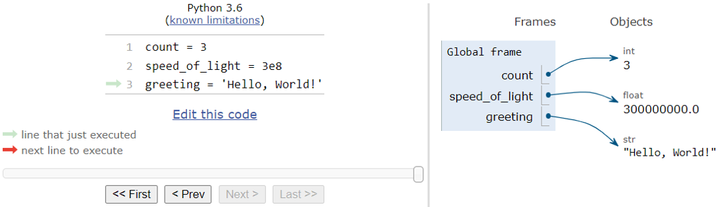
Figure 1. Python objects and variables. (Click image for full-size view.)
The right pane of Python Tutor shows the state of memory after running the last line of code (line 3). Python Tutor shows a visual representation of run-time state (stack frame contents such as variables, objects on heap, and pointer references).
The right pane is divided into the following sections:
- The heap is labeled Objects. Figure 1 shows three objects (or values) on the heap.
- The stack frames are shown under the label Frames. Figure 1 shows one stack frame called Global frame.
The link or association between variables and objects is shown either with an arrow or by using a text label such as idn (where n is a number) for the memory address of the object on the heap. Figure 1 shows associations using arrows, and this concept is explained in Section 2.5.3 Python Variable Model.
Keeping track of the objects or values associated with variables after each statement has been executed is called tracing a program. Tracing a program is useful for understanding how the program works and is a useful tool for finding errors in programs. You can use Python Tutor to trace a program since it shows a visual representation of Python objects after execution of each step.
In subsequent sections, the state of memory during or after program execution is visualized using snapshots of Python Tutor.
Since you can run the program one step at a time, forward as well as backward, you can use Python Tutor to understand the flow of execution (the order in which statements are executed) of the code.
2.5.2 C Variable Model
To understand variables in Python, it is useful to compare Python variables with C variables. In C, you must specify the data type of the variable followed by the name. For example, you create an integer variable whose value is 2 using the following assignment statement:
int x = 2;
As a result of executing this assignment statement, C does the following:
- Reserves enough space on the stack to store an integer
- Stores the integer value 2 at that memory address
- Links the variable name x with that memory address
In C, values are stored in variables. A variable is a named storage location, which stores a value of a particular type.
Figure 2 shows the C Tutor visualization of this assignment statement.
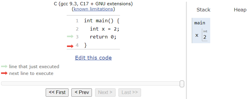
Figure 2. C variable model. (Click image for full-size view.)
2.5.3 Python Variable Model
As discussed in Section 2.4 Variables and Assignment Statement, Python variables are created using assignment statements. For example:
>>> x = 2
As a result of executing this assignment statement, Python does the following:
- Creates an int object on the heap to represent the integer value 2 (stores the integer value 2 in the object)
- Creates the variable x on the stack
- Links the variable x to the int object
Figure 3 shows the Python Tutor visualization of this assignment statement.
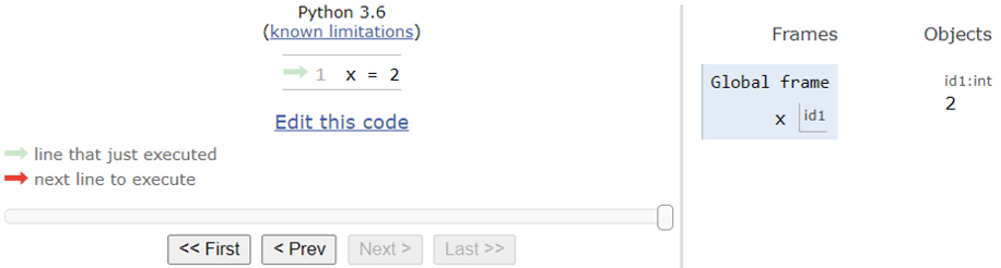
Figure 3. Python variable model. (Click image for full-size view.)
Python links the variable on the stack to the object on the heap by storing the address of the object (indicated in Figure 3 by the label id1) in the variable. The address of the object in memory is known as the object reference (see Introduction to Programming in Python). Therefore, a Python variable is a reference to an object.
Evaluating the variable name results in the value of the object and not the memory location of the object. For example:
>>> x = 2
>>> id(x)  # get memory address of object
140736114986784
>>> x
2
Therefore, you can use the name of a Python variable to refer to (or access) objects and can say that a Python variable is simply a name that refers to a value.
A Python variable is simply a name because, in contrast to a C variable, it does not store the actual object or value. It stores the memory address of the object. When a name is linked to an object, you can refer to the object by that name, but the data itself is stored within the object.
2.5.3.1 Visualizing Variables Using Arrows
In Figure 3, Python Tutor visualizes the link between the variable and the object by placing the address of the object (indicated by the label id1) inside the variable as well as next to the object.
Since the address of an object is not useful for programming, you can also use Python Tutor to visualize this link by drawing an arrow from the variable on the stack to the object on the heap.
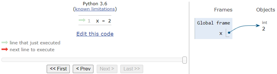
Figure 4. Python variable model using arrow. (Click image for full-size view.)
In subsequent sections, you will use Python Tutor to visualize the link between variables and objects using arrows. The arrow shows that the variable refers to the object.
2.5.4 Assignment and Binding
Section 2.4 Variables and Assignment Statement describes the syntax for the assignment statement: variable = value | expression
Since any object can be assigned to a variable, the syntax can be generalized to variable = object.
The updated syntax indicates that you can assign any type of object to a variable including primitive data types, compound data types, functions, modules, and files. You can create objects of different types and visualize them in Python Tutor. For example:
>>> my_list = [1, 2.4, True, None, 'Python']
>>> my_tuple = (1, 2.4, True, None, 'Python')
>>> my_dict = {'x': 1, (1, 1): [10, 20]}
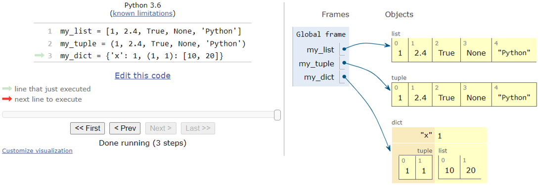
Figure 5. Assigning different object types to variables. (Click image for full-size view.)
As a result of executing each of these assignment statements, Python creates an object on the heap, creates a variable on the stack, and links the variable to the object.
Since Python links or binds a name to an object, assignment is also called binding (see The Python Language Reference: Naming and binding).
The assignment statement x = 2 has several equivalent meanings:
- Assign variable x to int object 2, or assign int object 2 to variable x.
- Bind variable x to int object 2.
- x is a reference to 2 or x refers to 2.
2.5.5 Properties of Objects
From the discussion in Section 2.5.3 Python Variable Model, you can see that:
- An object is a representation of a value in the memory of a computer.
- Every object has an identity, a type, and a value (see The Python Language Reference: Objects, values and types).
As discussed in Section 2.2.1 Numeric Types: int, float, and complex, Python objects can be created using literals. For example, if you evaluate the literal 2 at the Python prompt, then Python creates an object to represent the integer value 2:
>>> 2  # Create int object
2
The identity of an object is its address in the memory of the computer. Python automatically assigns each object a unique identity. The identify of an object never changes after it has been created. You can find the identify of an object by using the built-in id function:
>>> id(2)
140736114986784
The id function returns an integer representing the identify of an object.
The value of an object is the data-type value that it represents (see Introduction to Programming in Python). You can find the value of an object by evaluating it. Evaluating 2 creates an int object whose value is 2:
>>> 2  # Create int object and print its value
2
Evaluating 'Hello' creates a str object whose value is a sequence of characters:
>>> 'Hello'
'Hello'
Evaluating np.array([10, 20.5, 30]) creates an ndarray object whose value is an array of numbers:
>>> np.array([10, 20.5, 30])
array([10. , 20.5, 30. ])
As discussed in Section 2.2 Built-in Data Types, a data type or type is a set of values and a set of operations that can be performed on those values. The type of an object indicates the class to which it belongs, which you can find using the type function:
>>> type(2)
<class 'int'>
Python variables do not have types. Objects have types. Even though the assignment statement x = 2 binds the variable x to an int object that represents the value 2, for simplicity, it is often said that x is a variable of type int with value 2.
Since Python variables do not have types, you can reassign a variable to objects of different types. Reassigning a variable simply changes the object reference stored in the variable. After reassignment, the variable refers to a new object and stops referring to the older object:
>>> x = 2         # x is assigned to int object
>>> x
2
>>> id(x)
140717063999264

>>> x = 'Hello'   # x is reassigned to str object
>>> x
'Hello'
>>> id(x)
1767062621680

>>> x = [1, 2, 3]  # x is reassigned to list object
>>> x
[1, 2, 3]
>>> id(x)
1767050980544
As discussed in The Python Language Reference – Objects, values and types, after an object is created, its identity and type never change. The value of some objects can change and this is discussed in Section 2.5.5.1 Mutability of Objects.
The identity of an object does not change during the execution of the program. However, every time you run the program, Python might assign a different identity to the object.
2.5.5.1 Mutability of Objects
Mutable objects are objects whose value can change after they are created. For example, lists, NumPy arrays, and dictionaries are mutable. After a list is created, you can change any list element using its index:
>>> numbers = [10, 20, 30, 40]  # Create list object
>>> # Access first element of numbers list and assign to it 100
>>> numbers[0] = 100
>>> numbers
[100, 20, 30, 40]
The first element of the numbers list is updated. Therefore, the value of the list object has changed. Changing the value of an object is known as mutation.
Similar to lists, NumPy arrays are mutable:
>>> numbers = [10, 20, 30, 40]
>>> numbers = np.array([10, 20, 30, 40]) # Create ndarray object
>>> numbers[0] = 100
>>> numbers
array([100,  20,  30,  40])
Immutable objects are objects whose value cannot be changed after they are created. For example, strings are immutable. You cannot change the characters of an existing string. Trying to do so results in an error:
>>> greeting = 'Hello, World!'
>>> # Change first character of greeting
>>> greeting[0] = 'h'  # Immutable objects cannot be changed
Traceback (most recent call last):
  File "<stdin>", line 1, in <module>
TypeError: 'str' object does not support item assignment
In this error message, the "object" is the string and the "item" is the character you tried to assign.
Since lists are mutable and strings are immutable, most methods for transforming these objects result in the following:
- Modify the list argument (see Section 4.3.4 List Methods)
- Return a new string instead of modifying the string argument (see Section 4.3.5 String Methods)
2.5.5.2 Equality of Objects
Two Python variables can refer to the same object. For example, consider creating two variables and assigning the same string to them:
>>> str1 = 'TCAD'
>>> str2 = 'TCAD'
Here, Python creates two variables but a single string object. Both variables refer to the same string object as can be verified by using the id function and using Python Tutor.
>>> id(str1), id(str2)
(1766676883248, 1766676883248)
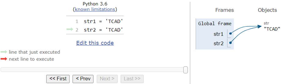
Figure 6. String equality. (Click image for full-size view.)
The operators is, is not, ==, and != are comparison operators (see Section 4.2.1 Comparison Operators). They return Boolean values.
The is operator tests for identity equality (reference equality). Two objects are identical if they have the same identity or the same memory address. So, it tests whether two variables refer to the same object. For example:
>>> str1 is str2
True
If the identities of two objects differ, then it returns False:
>>> str1, str2, str3 = 'TCAD', 'TCAD', 'Python'
>>> str1 is str3
False
The is not operator is used to test whether two variables refer to different objects:
>>> str1, str2, str3 = 'TCAD', 'TCAD', 'Python'
>>> str1 is not str2, str1 is not str3
(False, True)
The == operator tests for value equality (whether two objects represent the same value), and the != operator tests for value inequality. Two objects are said to be equivalent if they represent the same value. Obviously, this holds true for the two string objects str1 and str2 but not for str1 and str3:
>>> str1 == str2, str1 == str3
(True, False)
Python created a single (immutable) str object as a result of the following assignment statements:
str1 = 'TCAD'
str2 = 'TCAD'
However, when you assign a list, tuple, or NumPy array containing the same values to two variables, Python creates a new list, tuple, or NumPy array, respectively. For example:
>>> x = [10, 20, 30]
>>> y = [10, 20, 30]
>>> x == y, x is y
(True, False)
Here, x is y is False even though all corresponding elements in the two lists are the same. The two list objects are equivalent since they contain the same values. However, they are not identical since they are at different memory addresses.
Figure 7 shows the Python Tutor visualization of the two lists.
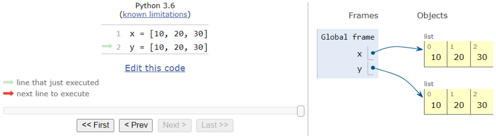
Figure 7. List equality. (Click image for full-size view.)
In the case of NumPy arrays, you can check for identity equality and value equality by using the is operator and the numpy.array_equal function, respectively:
>>> x = np.array([10, 20, 30])
>>> y = np.array([10, 20, 30])
>>> x is y, np.array_equal(x, y)
(False, True)
2.5.5.3 Aliasing, Assignment, and Mutable Objects
If a single object is associated with two different variables, then you can refer to the object using either one of the variable names. This is known as aliasing and the names are known as aliases. For example, in Section 2.5.5.2 Equality of Objects (and Figure 6), you saw that both str1 and str2 refer to the same string object 'TCAD'. Here, str1 and str2 are aliases.
Assigning one variable to another does not copy the contents from one variable to another. It copies the object reference (memory address of the object). After assignment, the two variables refer to the same object. So, assignment creates aliases.
For example, create a list object and assign it to a variable x:
>>> x = [10, 20, 30]
Next, assign the variable x to a new variable y:
>>> y = x # Assigns id of x to y
Instead of creating a new list object, copying the contents of list x to the new list object, and assigning the new list object to y, assigning y to x copies the memory address of x into y. Both variables refer to the same list object. As a result, x and y are aliases to the same list object as can be verified using the is operator and Python Tutor:
>>> x is y  # verify that x and y are aliases
True
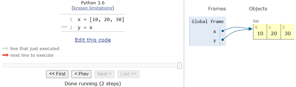
Figure 8. Aliased lists. (Click image for full-size view.)
Since lists are mutable, you can modify the same list object using either one of the aliases:
>>> y[0] = 1  # Change y
>>> y
[1, 20, 30]
>>> x  # x is also changed
[1, 20, 30]
This is true not only for lists, but also for any type of object. Instead of copying the content of an object into a new object, assignment creates an alias to the same object. If aliased objects are mutable, then you can modify the same object using either one of the aliases. For example, even NumPy arrays are mutable and the behavior of aliased NumPy arrays is similar to that of aliased lists:
>>> x = np.array([10, 20, 30])
>>> y = x     # Both x and y refer to same object
>>> x is y
True
>>> y[0] = 1  # Changing y changes x
>>> x
array([ 1, 20, 30])
This behavior of aliased mutable objects might lead to errors and should be avoided. It is less error prone to have only a single reference to a mutable object.
2.5.5.4 Copying Objects
You can prevent aliasing by copying the contents of an object into a new object. In the case of sequences such as lists, tuples, and strings, you can create copies using the slicing operation (see Section 4.3.2 Slicing). A slice of a sequence is a portion of the sequence. You can create a slice containing the entire sequence using the syntax: sequence[:]
You can create a copy of the sequence by assigning this slice. The contents of both sequences are the same. For example:
>>> x = [10, 20, 30]
>>> # Create a slice of entire sequence and assign to z
>>> z = x[:]
>>> z
[10, 20, 30]
You can verify that the two lists are equivalent but not identical:
>>> x == z, x is z
(True, False)
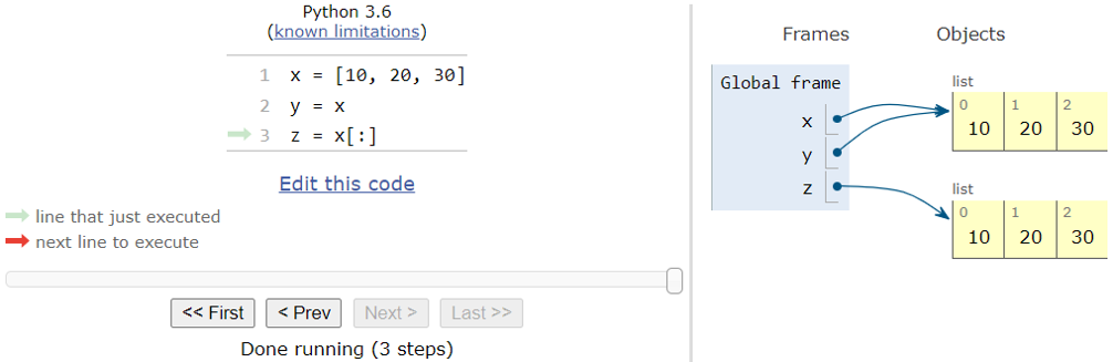
Figure 9. Copying lists. (Click image for full-size view.)
Slicing does not create a copy of a NumPy array but creates a view of the array (see Section 4.3.2 Slicing):
>>> x = np.array([10, 20, 30])
>>> z = x[:]  # Assign a slice of x to  z
>>> z[0] = 0  # Change z
>>> x         # x is also changed
array([ 0, 20, 30])
You can make copies of NumPy arrays by using the numpy.ndarray.copy() method. The copy() method is defined in the ndarray class, which is defined in the NumPy package. It acts on a NumPy array (for more details, see Section 3.3.1.4 Referencing Methods):
>>> x = np.array([10, 20, 30])
>>> # Make a copy of array x and assign to y
>>> y = x.copy()
>>> # Test for identity equality and equivalence
>>> y is x, np.array_equal(x, y)
(False, True)
Similarly, you can use the dict.copy() method to copy dictionaries.
The Python copy module contains functions for copying not only sequences but also any type of object. You can also use the copy module to copy user-defined types. For example, see Section 3.3.2.3 Mutability, Aliasing, and Copying.
2.6 Introduction to Looping
Executing a sequence of statements repeatedly is called looping or iteration. You can perform iteration in Python using the for statement and the while statement.
The Python for statement works like the Tcl foreach command (but not like the Tcl for command). It iterates over all the elements of a sequence, in the order in which they appear in the sequence. Therefore, you can execute the same sequence of statements once for each item in a sequence.
The syntax of the for loop is:
for <variable> in <sequence>
    body
The first statement is the header and the subsequent statements form the body of the for statement. All statements in the body of the for loop are indented.
The following program sums over a list of numbers:
# Script: loop_for.py
numbers = [11, 22, 33, 43]
counter, total = 1, 0
for num in numbers:
    print(f'Iteration number: {counter}')
    total += num
    print(f'Partial sum: {total}')
    counter += 1

print(total)

> gpythonsh loop_for.py
Iteration number: 1
Partial sum: 11
Iteration number: 2
Partial sum: 33
Iteration number: 3
Partial sum: 66
Iteration number: 4
Partial sum: 109
109
The for statement steps through the given sequence, here the numbers list, and executes all the statements in the body of the loop. The current element of the list is assigned to a variable (here num). During the first iteration, the first element (11) of the list is assigned to the variable num. During each subsequent iteration, the next element of the list is assigned to the variable (num). The iterations continue until the last element of the sequence is assigned.
Here, the variable counter is used to keep track of the iteration number.
Additional looping-related concepts are discussed in Section 4.1 More on Looping.
Copyright © 2022 Synopsys, Inc. All rights reserved.