
Python Language
3. Modules, Functions, and Classes
3.1 Python Modules and Packages
3.2 Functions
3.3 Objects and Classes
Objectives
- To introduce Python modules, packages, functions, objects, and classes.
3.1 Python Modules and Packages
The scripts discussed here are available in the directory
Applications_Library/GettingStarted/python/py_basics. The code examples
that must be entered at the interactive prompt are also available in this
Sentaurus Workbench project.
Click to view the primary file
python_pyt.py.
To easily reuse functionality, Python allows you to structure code into modules and packages. A Python module is a file containing a collection of related variables, functions, and classes. A Python package is a collection of related Python modules.
3.1.1 Available Modules
Several types of Python modules and packages are available:
- Built-in
- Python Standard Library
- Python packages for scientific computing
- Sentaurus Visual Python packages
3.1.1.1 Built-in Module
As part of the built-in module, the Python interpreter has a number of:
- Constants (see The Python Standard Library: Built-in Constants)
- Functions (see The Python Standard Library: Built-in Functions)
- Types or classes (see The Python Standard Library: Built-in Types)
Unlike other modules discussed in the next sections, there is no need to explicitly import the built-in module since Python automatically imports it on startup.
Some of the built-in constants and built-in types are discussed in Section 2.2 Built-in Data Types. The built-in functions are discussed in Section 3.2.1.1 Using Built-in Functions.
3.1.1.2 Python Standard Library
The Python Standard Library is distributed with Python. It contains many modules for common programming tasks, for example:
- Scientific computing: math, cmath, statistics, and random modules
- Copying objects: copy module
- Logging system: logging module
- Debugging: pdb module
- File pathname matching: glob module
- String pattern matching: re module
- Operating system interfaces: os module
- Unit testing framework: unittest module
- GUI development: tkinter module
- Printing arbitrary Python data structures in a more readable way: pprint module
For an introduction to the modules in the Python Standard Library, see The Python Tutorial: Brief Tour of the Standard Library and The Python Tutorial: Brief Tour of the Standard Library — Part II.
The following Python Standard Library modules are useful for scientific computations:
- math module includes mathematical constants and functions.
- cmath module includes mathematical functions for complex numbers.
- statistics module includes mathematical statistics functions.
- random module is used for generating pseudorandom numbers.
3.1.1.3 Python Scientific Computing Stack
Python has many packages for scientific computation, but they are not included in the standard Python distribution. They must be installed separately. These packages are part of the Python Scientific Computing stack. The TCAD Python distribution includes many of these packages such as:
- NumPy (Numerical Python) provides the multidimensional array object and fast array operations. Other packages such as SciPy and pandas use multidimensional arrays to store data. It allows for vectorized operations, which are discussed in Section 3.1.4.2 Scalar-Oriented Versus Vectorized Code.
- SciPy (Scientific Python) provides algorithms for differentiation, integration, interpolation, statistics, and many other scientific computation problems.
- pandas provides the DataFrame object, which can be used to represent tabular data. It is useful for working with datasets. Similar to NumPy, it provides many functions for processing tabular data. It can be used to read and process data from CSV files. See Section 5.3 Sentaurus Visual: Loading CSV File Using pandas for an introduction to pandas.
You can see a complete list of the included packages by entering:
% gpythonsh -m pip list
3.1.1.4 Sentaurus Visual Python Packages
Sentaurus Visual Python Mode consists of the following packages:
- The svisual package contains Python functions for visualizing and analyzing TCAD simulation results in both interactive mode and batch mode (see Section 6.7 Sentaurus Visual in Python Mode).
- The svisualpylib package contains modules for extracting device parameters such as the Extraction module (extract), RF Extraction module (rfx), Harmonic Balance module (hb), and IFM module (ifm). These are discussed briefly in Section 6.8 Sentaurus Visual Python Extraction Modules and Tcl Extraction Libraries.
3.1.2 Using Modules
In some sense, you can think of a Python module as a library. You must load modules using the import statement before using them. For example, the math module is available as the file math.py. You can import the entire math module using the import statement followed by the name of the module without the file extension .py.
>>> import math # Now, the entire math module is available
After importing a module, you can view the functions, methods, and constants defined in the module using the dir function and can see help about the entire module or specific functions by using the help function (see Section 1.4 Online Help).
It is common to import modules and rename them using the as keyword to more convenient shorter names. For example, the following statement imports the entire NumPy package and renames it to np:
>>> import numpy as np
Since you need to prepend the function name with the module name (see Section 3.1.2.1 Modules as Objects for an explanation of dot notation), the modules are renamed in order to shorten their names. To use functions from the NumPy package such as the array function, you must now write np.array instead of numpy.array.
Similarly, by default, Sentaurus Visual Python imports the svisual package using:
import svisual as sv
This statement imports the entire svisual module and renames it to sv.
Instead of importing the entire module, it is also common to import only the required functions and variables from a module. For example, the following statement imports only the degrees function and the constant pi from the math module:
>>> from math import degrees, pi
Now, you can access them without prepending their names with the module name:
>>> radius = 1
>>> # Use the name pi instead of math.pi
>>> pi * (radius ** 2), 2 * pi * radius
(3.141592653589793, 6.283185307179586)
>>> # Use the name degrees instead of math.degrees
>>> degrees(pi)
180.0
3.1.2.1 Modules as Objects
Python modules are objects. The statement import module_name creates a module object whose name is module_name. For example, executing the import math statement creates a module object called math:
>>> import math
>>> type(math)
<class 'module'>
You can visualize in Python Tutor the state of memory after the execution of the import statement.
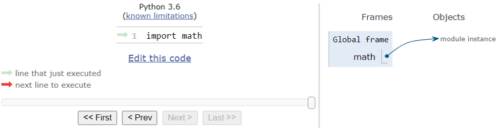
Figure 1. Module as object. (Click image for full-size view.)
Figure 1 shows that, as a result of executing an import statement (for example, import math), Python does the following:
- Creates a module object on the heap
- Adds a variable to the stack, whose name is the name of the module (math)
- Stores the address of the module object in the variable
Python stores the contents of the module in the module object as attributes (attributes are defined in Section 3.3 Objects and Classes). The variables defined inside a module are stored as data attributes, and functions are stored as methods. Therefore, to access the variables and functions defined in a module, you must use dot notation in which the name of the module is prepended to the name of the variable or function:
module.<variable>
module.<function()>
For example:
>>> import math
>>> # access constant pi defined in math module
>>> math.pi
3.141592653589793

>>> # Some other constants defined in math library
>>> math.e, math.tau, math.inf, math.nan
(2.718281828459045, 6.283185307179586, inf, nan)

>>> # Calculate area and circumference of a circle of radius 1 unit
>>> radius = 1
>>> math.pi * (radius ** 2), 2 * math.pi * radius
(3.141592653589793, 6.283185307179586)
3.1.3 Mathematical Constants
The math module defines various mathematical constants and functions. All the constants such as math.pi and math.e are implemented as variables since Python does not support constants. Table 1 lists some of these mathematical constants as well as constants available in Python and in the NumPy package (see NumPy API Reference - Constants).
| Variable | Definition |
|---|---|
| _ | Value of last evaluated expression; defined only in interactive mode (not a mathematical constant) |
| 1j | \( √{-1} \) (not a mathematical constant) |
| math.pi | Mathematical constant \( π \) |
| math.tau | \( τ = 2 π \) |
| math.e | Mathematical constant \( e \) |
| float('nan'), math.nan, numpy.nan | Not a number (NaN); obtained as a result of invalid operations |
| float('inf'), math.inf, numpy.inf | \( + ∞ \) |
| -float('inf'), -math.inf, -numpy.inf, numpy.NINF | \( - ∞ \) |
As mentioned in Section 2.2.1 Numeric Types: int, float, and complex, to create complex numbers from expressions, you need to multiply the expression by the imaginary unit 1j or 1J. For example, you can represent the complex number \( π j\) in Python as follows:
>>> import math
>>> math.pi * 1j
3.141592653589793j
3.1.4 Physical Constants: scipy.constants Module
Physical constants are available in the constants module of the SciPy package (scipy.constants module). Some of these are listed in Table 2. This module also provides conversion factors from different units to SI units. However, it does not support unit algebra.
| Variable | Definition |
|---|---|
| c, speed_of_light | Speed of light in vacuum |
| h, Planck | Planck's constant \( ℎ \) |
| hbar | \( ℏ = ℎ / {2 π} \) |
| e, elementary_charge | Elementary charge |
| k, Boltzmann | Boltzmann constant |
| epsilon_0 | Vacuum permittivity |
| mu_0 | Vacuum permeability |
As with other modules, you must import the scipy.constants module before using the constants. Each constant is defined as a variable (since Python does not have constants), and you use the variable name to access the constant:
>>> import scipy.constants as const
>>> const.epsilon_0  # Access vacuum permeability
Calling the dir function by passing const as a parameter returns a list of the names of physical constants, functions, and names of non-SI units defined in the scipy.constants module:
>>> dir(const)
['Avogadro', 'Boltzmann', 'Btu', 'Btu_IT', 'Btu_th', 'ConstantWarning',
'G', 'Julian_year', 'N_A', 'Planck', 'R', 'Rydberg', 'Stefan_Boltzmann'
...
'u', 'unit', 'value', 'week', 'yard', 'year', 'yobi', 'yotta', 'zebi',
'zepto', 'zero_Celsius', 'zetta']
Some constants such as the speed of light in vacuum have a single letter name as well as a more descriptive one:
>>> const.c, const.speed_of_light
(299792458.0, 299792458.0)
CODATA physical constants and functions in the scipy.constants module are discussed in Section 4.4 More on scipy.constants Module.
3.1.4.1 Unit Conversion
Conversion factors are available for converting the following:
- Non-SI unit to an SI unit of a physical quantity
- SI unit with prefix to SI unit
You can access the conversion factors using the variable name of the unit or prefix. For example, 1 eV = 1.602 × 10⁻¹⁹ J. To access the conversion factor for converting from eV to J, use the variable name eV:
>>> const.eV  # one electron volt in joules
1.602176634e-19
>>> # Conversion factor for converting micrometer to m
>>> const.micron # 1 micrometer = 1e-6 m
1e-06
You can convert from a different unit to an SI unit by multiplication:
>>> 5 * const.nano  # Convert 5 nm to m
5e-09
You can convert from an SI unit to a non-SI unit by division:
>>> 5e-9 / const.nano  # Convert 5e-9 m to nm
5.0
The variables corresponding to SI units are not defined since their conversion factors are 1. For example, there is no variable called m for meter.
Here is an example of using the physical constants and conversion factors from the scipy.constants module. The long-wavelength cutoff, \( λ_c \), of a photodiode is limited by the semiconductor bandgap, \( E_g \), and is given by: \[ λ_c = {ℎ c} / E_{g} \] where:
- $ ℎ $ is Planck's constant.
- $ c $ is the speed of light in vacuum.
The band gap and the cutoff wavelength are usually specified in units of eV and nm, respectively. You can compute the cutoff wavelength in units of nm for GaAs with $E_{g}$ = 1.424 eV using the following script:
# Script: eg2lambda.py
import scipy.constants as const

bandgap_ev = 1.424  # GaAs bandgap in eV
# Convert bandgap unit from eV to J
bandgap_joule = bandgap_ev * const.eV
lambda_meter = const.h * const.c / bandgap_joule  # wavelength in m
lambda_nm = lambda_meter / const.nano             # wavelength in nm
print(f'cut-off wavelength: {lambda_nm:.2f} nm')
> gpythonsh eg2lambda.py
cut-off wavelength: 870.68 nm
3.1.4.2 Scalar-Oriented Versus Vectorized Code
Suppose you want to compute the cutoff wavelength of several semiconductors. You can do this by using either a scalar-oriented loop-based approach or a vectorized array-based approach. The following code illustrates the scalar-oriented loop-based approach:
# Script: eg2lambda_list.py
import scipy.constants as const

# Specify band gaps of Ge, Si, and GaAs in a list
bandgap_ev = [0.661, 1.12, 1.424]

lambda_nm = []  # Create empty list
for eg in bandgap_ev:
    bandgap_joule = eg * const.eV
    lambda_meter = const.h * const.c / bandgap_joule
    lambda_nm.append(lambda_meter / const.nano)

print(f'cut-off wavelength: {lambda_nm} nm')

> gpythonsh eg2lambda_list.py
cut-off wavelength: [1875.7064815915317, 1107.0017717250023, 870.6755507949458] nm
In the scalar-oriented loop-based approach, you do the following:
- Store all the band gaps in a list.
- Create an empty list to store the wavelengths.
- Loop over the individual band gaps using the for statement and:
- Compute the individual cutoff wavelengths using scalar arithmetic operations.
- Append these individual wavelengths to the list of wavelengths using the list.append() method, which adds an item to the end of the list (see Section 4.3.4 List Methods).
Here is the vectorized version of the previous code:
# Script: eg2lambda_array.py
import numpy as np
import scipy.constants as const

# Set the precision for printing floating-point numbers in NumPy objects
np.set_printoptions(precision=2)

# Specify band gaps of Ge, Si, and GaAs in 1D array
bandgap_ev = np.array([0.661, 1.12, 1.424])

# Use elementwise scalar multiplication to convert all band gaps
# from eV to SI unit
bandgap_joule = bandgap_ev * const.eV
# Compute wavelength in [m] using elementwise inverse of array
lambda_meter = const.h * const.c / bandgap_joule
lambda_nm = lambda_meter / const.nano

print(f'cut-off wavelengths: {lambda_nm} nm')

> gpythonsh eg2lambda_array.py
cut-off wavelengths: [1875.71 1107.    870.68] nm
In the vectorized array-based approach, you do the following:
- Store all the band gaps in a 1D array.
- Use vectorized operations to compute the cutoff wavelength for all the band gaps in a single statement.
The results of vectorized computation are stored in an array.
Using code that uses vectorized operations instead of loops is called vectorized code, and using array-based vectorized code instead of scalar-oriented loop-based code is called vectorization. Vectorized code has several advantages over the corresponding scalar-oriented loop-based code:
- It is easier to implement and understand vectorized code since it looks similar to mathematical expressions.
- Programs using vectorized code are more concise since they do not use loops.
- Vectorized code usually runs faster than loop-based code.
3.2 Functions
A function is a named sequence of statements that performs a computation or another task. For example, the following are built-in functions:
- The abs function computes the absolute value of a number.
- The print function displays a message.
- The type function displays the type of an object.
3.2.1 Using Functions
To use functions for performing computations, you must invoke or call them. A function call is an expression containing the function name followed by a pair of parentheses containing zero or more comma-separated expressions called arguments. Arguments allow you to pass information to the function.
Here is an example of a function call with a single argument:
>>> abs(1 + 1j)  # Call abs function with argument 1 + 1j
1.4142135623730951
Similar to all expressions, a function call evaluates to a value (here, 1.4142135623730951).
When Python evaluates a function call, it executes the statement inside a function. After it is called, the function uses the arguments to perform the computation or task, and then returns to the program step from which it was called. Going back to the calling program is called returning from the function. As part of the return operation, functions send results back to the calling program. This result is called the return value.
In many ways, Python functions are similar to mathematical functions. They take input (arguments) and return an output (return value).
In contrast to mathematical functions, Python functions can return not only numeric objects but also any other type of object such as strings or lists. Some functions such as the print function and many other list methods (see Section 4.3.4 List Methods) return the value None. For example:
>>> print(print('Hello, World!'))
Hello, World!
None
Here, the outer print function call displays the None returned by the inner print function call.
>>> type(print('Hello, World'))
Hello, World!
<class 'NoneType'>
Both these function calls are examples of composing functions (see Section 3.2.1.3 Composing Functions).
3.2.1.1 Using Built-in Functions
As discussed in Section 3.1 Python Modules and Packages, many Python functions are available in modules and, before using any of these functions, you need to import the respective module. The Python interpreter has several functions as part of the built-in module, which is always available. There is no need to import it.
You have already used built-in Python functions such as print, help, type, and id. Some of the useful built-in mathematical functions are abs, min, max, pow, round, and sum. These functions are documented in The Python Standard Library: Built-in Functions.
You can see information about the arguments and return value of a function by using the help function:
>>> # Get help on abs function
>>> help(abs)  # call help function with argument abs
Help on built-in function abs in module builtins:

abs(x, /)
    Return the absolute value of the argument.
3.2.1.2 Using Mathematical Functions
Various mathematical functions are available in the math module, cmath module, and NumPy package.
As discussed in Section 3.1.2.1 Modules as Objects, before invoking functions defined in modules, you need to:
- Import the module
- Use dot notation to call the functions
For example:
>>> import math
>>> # Call sin function defined in math module
>>> math.sin(math.pi / 2)
1.0
>>> # Calculate pi using inverse sin function
>>> pi = 2.0 * math.asin(1.0)
>>> print(f'pi = {pi:.5f}')
pi = 3.14159
>>> # Verify Euler's identity
>>> import math, cmath  # Importing multiple modules
>>> cmath.exp(math.pi * 1j) + 1
1.2246467991473532e-16j
You also need to use dot notation when requesting help for functions in modules:
>>> help(math.sin)  # help on sin function in math module
Help on built-in function sin in module math:

sin(x, /)
    Return the sine of x (measured in radians).
1.0
3.2.1.3 Composing Functions
The syntax for composing functions in Python is similar to the mathematical notation for composing functions. For example, you can compute $e^{\ln{e}$ using:
>>> import math
>>> math.exp(math.log(math.e))
2.718281828459045
The order of evaluation is as expected. The innermost function is executed first. The return value of the inner function is passed as the argument to the outer function. Here is another example of composition using functions:
>>> # Compute maximum of 2, 3, 4 and then square the maximum
>>> pow(max(2, 3, 4), 2)
16
3.2.1.4 NumPy Universal Functions
The mathematical functions in the built-in, math, and cmath modules operate on a single value. For example, you can use the math.degrees function to convert an angle from radians to degrees:
>>> import math
>>> math.degrees(math.pi)
180.0
NumPy has a vectorized version of mathematical and statistical functions called universal functions (ufunc for short), which can be used to perform computations on several values at the same time. A ufunc is a function that performs elementwise operations on NumPy arrays and returns a new array. For example:
>>> import numpy as np
>>> # Convert several angles from degrees to radians
>>> angle_radians = np.array([0, np.pi/4, np.pi/2, 3*np.pi/4, np.pi])
>>> np.rad2deg(angle_radians)
array([  0.,  45.,  90., 135., 180.])

>>> # Compute hypotenuse of a right-angled triangle
>>> side1 = np.array([1, 2, 3])
>>> side2 = np.array([5, 5, 6])
>>> np.hypot(side1, side2)
array([5.09901951, 5.38516481, 6.70820393])
The ufuncs operate on scalars as well. For example:
>>> np.sin(np.pi/2)
1.0
NumPy has functions that handle complex numbers (see Handling complex numbers):
>>> z = np.array([1 + 1j, -1 + 1j, -1, -1j, -1 - 1j])
>>> np.real(z)  # Real part of array of complex numbers
array([ 1., -1., -1., -0., -1.])
>>> np.conjugate(z)  # conjugate of array of complex numbers
array([ 1.-1.j, -1.-1.j, -1.-0.j, -0.+1.j, -1.+1.j])
NumPy also supports not a number (NaN) values. It has functions that operate on arrays with NaN values. For example, the numpy.sum function computes the sum of all array elements, but it does not ignore NaN values:
>>> x = np.array([1, 2, np.nan, 3])
>>> np.sum(x)
nan
The corresponding numpy.nansum function also computes the sum of all array elements but treats NaN values as zero:
>>> np.nansum(x)
6.0
3.2.2 User-Defined Functions
You can create your own functions using the def keyword. Here is the syntax for a function definition:
def <function_name>(<formal parameters>):
    code block
    return <expression>
The syntax is discussed using an example: define a function for computing the resistivity $ρ$ of an n-type uniformly doped semiconductor using:
\[ ρ = {1}/{e μ_n N_D} \]
where:
- $e$ is the elementary charge.
- $μ_n$ is the electron mobility.
- $N_D$ is the donor concentration.
The following code implements this computation using the resistivity function:
# Script: resistivity.py
# Import physical constants from scipy.constants module
import scipy.constants as const

# Define function
def resistivity(nd, mobility_n):
    """Compute resistivity of n-type semiconductor.

    :param nd: donor concentration [1/cm^3]
    :param mobility_n: electron mobility [cm2/(V-s)]
    :return: resistivity [Ohm-cm] of n-type semiconductor

    """
    sigma = const.e * mobility_n * nd
    rho = 1/sigma
    return rho
As discussed in The Python Tutorial: Defining Functions:
- A function definition has two parts:
- The header is the first line of the definition.
- The body is the rest of the definition.
- The header consists of the def keyword, followed by the name of the function and the signature of the function, which is the parenthesized list of formal parameters, here (nd, mobility_n). The parameters receive the value of the arguments used in a function call.
- All statements after the def statement are indented and form the body of the function. The colon (:) after the def statement and the indented body tells the Python interpreter that the indented statements belong to the resistivity function. The indentation determines whether the code belongs to the defined function or to any remaining code.
- The first statement of the function body can optionally be a triple-quoted string; this string
is the documentation string (or docstring) of the function. Unlike # comments,
Python saves the docstring and displays it when you call the help function with the
function name as the argument. The help message shows the function name and the parameters along
with the docstring:
> gpythonsh -m IPython -i resistivity.py In [1]: help(resistivity) Help on function resistivity in module __main__: resistivity(nd, mobility_n) Compute resistivity of n-type semiconductor. :param nd: donor concentration [1/cm^3] :param mobility_n: electron mobility [cm2/(V-s)] :return: resistivity [Ohm-cm] of n-type semiconductor - The return statement is used to return the value of the expression after the return keyword. The return value can be any Python data type such as string or list. If the return statement is not included in the function definition, then by default, the function returns None. So, Python functions always return a value.
- A function can be defined anywhere in a script, but it can be called only after being defined.
The statements inside a function definition are not executed immediately after the function definition. When Python executes the function definition, it creates a function object and stores a function definition in the object as shown in the following Python Tutor visualization.
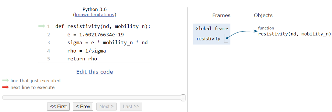
Figure 2. Function as object. (Click image for full-size view.)
Python functions are objects of type function:
In [2]: type(resistivity)
Out[2]: function
To compute the resistivity of n-type Si with $N_{D} = 10^{17} cm^{-3}$ and $μ_{n} = 700 \ {cm}^{2}/{V.s}$, you must call the resistivity function with these arguments:
In [3]: resistivity(1e17, 700)
Out[3]: 0.08916441534943947
In this example, you passed arguments to the resistivity function using positional parameters. You can also pass arguments to functions using keyword arguments or a combination of both positional and keyword arguments. Keyword arguments can be used to define default parameter values. For more details, refer to The Python Tutorial: Special parameters. These concepts are also explained in the appendix of the project documentation for Applications_Library/CMOS/CMOS_Characterization.
3.2.3 Local and Global Variables
The variables that are defined inside a function and parameters exist only inside the function. You can access them only from inside the function. Therefore, they are called local variables. You cannot access local variables from outside the function. For example, you defined the variables sigma and rho inside the resistivity function. These cannot be accessed outside the function. Attempting to do so results in an error:
In [4]: sigma
---------------------------------------------------------------------------
NameError                                 Traceback (most recent call last)
<ipython-input-4-bc0b719fd29e> in <module>
----> 1 sigma

NameError: name 'sigma' is not defined
Variables defined outside a function are called global variables. For example, in the resistivity.py script, the variable const.e is a global variable created as a result of importing the scipy.constants module. Global variables can be accessed inside the function (for example, in the statement sigma = const.e * mobility_n * nd) as well as outside the function:
In [5]: const.e
Out[5]: 1.602176634e-19
You can find global variables using the built-in globals function. It returns a dictionary whose keys include the global variables and their values:
> gpythonsh

>>> x, y = 1, 2
>>> globals()
{'__name__': '__main__', '__doc__': None, '__package__': None,
'__loader__': <class '_frozen_importlib.BuiltinImporter'>, '__spec__': None,
'__annotations__': {}, '__builtins__': <module 'builtins' (built-in)>,
...
'x': 1, 'y': 2}
3.2.4 Returning Multiple Values
You can use Python functions to return multiple values by using a sequence type such as list, tuple, or NumPy array, or by using a dictionary. For example, you can use the built-in divmod function to perform integer division. It returns both the quotient and the remainder as a tuple:
>>> divmod(5, 3)
(1, 2)
3.3 Objects and Classes
Here is a summary of what has been covered about objects and classes so far:
- Everything (including data) is represented by objects in Python.
- Objects have an identity, a type, and a value. The type and identity of an object do not change during the execution of a program. The value of mutable objects can change.
- Instead of copying the content of an object into a new object, assignment creates an alias to the same object.
- Objects have attributes. There are two types of attribute: data attributes and methods.
- Each object is created from a class.
- Python has several built-in classes. You can create your own data types and these are called user-defined classes.
According to the Python Glossary:
A class is a template for creating user-defined objects. Class definitions normally contain method definitions which operate on instances of the class.
An object is any data with state (attributes or value) and defined behavior (methods).
Since an object is constructed from a class, a class serves as a template or blueprint for creating an object. Since a class can be used to construct many objects, the created objects are also called instances of the class and creating an object is called instantiation.
3.3.1 Using Objects
So far, you have been using objects from built-in classes. All data types, including numbers, Booleans, NoneType, strings, and various other data structures such as lists and NumPy arrays are objects. For example, the documentation for the type complex reads as follows:
class complex([real[, imag]])
    Return a complex number with the value real + imag*1j or
    convert a string or number to a complex number.
    ...
It shows that complex is a class.
3.3.1.1 Creating Objects
There are several ways of creating objects of built-in classes in Python:
- Literals
- Special syntax
- Constructor
You have been using literals and the special syntax for creating objects (for example, see Section 2.2 Built-in Data Types). Executing an expression containing literals creates an object that represents the specified value. For example, executing the literal 2 + 3j creates a complex object to represent the complex number $2 + 3i$, whose real part is 2 and imaginary part is 3:
>>> z = 2 + 3j  # Create complex object using literals
>>> z
(2+3j)
Python has a special syntax for creating objects that represent data structures such as lists, tuples, and dictionaries:
- To create lists or tuples, enclose values inside brackets or parentheses, respectively (see Section 2.2.5.2 Lists and Tuples).
- To create dictionaries, enclose key–value pairs inside braces (see Section 2.2.6 Introduction to Dictionaries).
All objects, both built-in and user-defined, can be created using the constructor for the class. A constructor is a function that creates an object. Its name is the name of the type of object that you want to create.
Calling the constructor of a built-in type creates a new object of that type. The name of the constructor is the class name. For example, a list object can be created using the list constructor and a complex object can be constructed using the complex constructor.
You can create an object to represent the complex number $2 + 3i$ using the complex constructor:
>>> z = complex(2, 3)  # Create complex object using constructor
>>> z                  # Get value of z
(2+3j)
>>> type(z)
<class 'complex'>
The class of z is complex.
3.3.1.2 Attributes: State and Behavior of Objects
The attributes of an object are defined in the class. There are two types of attribute:
- data attributes: The variables defined inside a class are called data attributes since they are used to store data. Each time you create a new object, Python assigns a set of data attributes to the object. The set of values contained in these data attributes is known as the state of an object. Mutating an object changes the value of the data attributes and, therefore, its state.
- methods: The functions defined inside a class are called methods. They are used to perform operations on data attributes of instances of the class. The set of operations that can be performed on an object is known as the behavior of an object.
Since data is stored in objects, you can say that an object is any data with a state (data attributes and their values) and defined behavior (methods).
Before using objects, either built-in or those available in other Python packages, you need to know about the following:
- The operations that can be performed on the data attributes of an object
- How to perform the operations, that is, the required arguments and the syntax:
- Operator
- Function call
- Method call
- The result of the operation, that is, whether it mutates the object, returns a new object, or simply provides information about the object
To use objects for performing computations, you do not need to know the implementation details about the data attributes or the methods. Implementation details are in the class implementation, which is hidden from users.
You can find the attributes (both data attributes and methods) of a class using the dir function:
>>> print(dir(z))
['__abs__', '__add__', ..., 'conjugate', 'imag', 'real']
Here, imag and real are data attributes and conjugate is a method. The names surrounded by double underscores (__) are special methods in Python. They are informally known as dunder (double underscores) methods (see Section 3.3.1.5 Referencing Dunder Methods (Advanced)).
You can request help for these attributes by using dot notation, which is explained in the next section:
>>> help(z.conjugate)
Help on built-in function conjugate:

conjugate(...) method of builtins.complex instance
    complex.conjugate() -> complex

    Return the complex conjugate of its argument. (3-4j).conjugate() == 3+4j.

Help on built-in function conjugate:

conjugate(...) method of builtins.complex instance
    complex.conjugate() -> complex

    Return the complex conjugate of its argument. (3-4j).conjugate() == 3+4j.
The next sections explain how to use these attributes.
3.3.1.3 Referencing Data Attributes
You have already seen that if a primitive object such as a number is assigned to a variable, you can access the value of the object using the name of the variable:
>>> x = 2
>>> x
2
If a data structure such as list is assigned to a variable, then you can access an element using the variable name followed by the index of the element inside brackets:
>>> x = [2, 3]
>>> x[0], x[1]  # Access list elements
(2, 3)
Accessing the data attributes of an object is similar to accessing list elements. Instead of using an integer (the index), you must use the name of the data attribute and, instead of using brackets, you must use a period: object.<data_attribute>
This syntax for accessing or referencing attributes is also known as dot notation since it contains a period (.). For example, the complex object has the following data attributes:
- real represents the real part of complex numbers.
- imag represents the imaginary part of complex numbers.
You can use dot notation to access them:
>>> z = 2 + 3j
>>> z.real, z.imag
(2.0, 3.0)
Trying to access an attribute that is not defined for an object results in an error:
>>> z.con
Traceback (most recent call last):
  File "<stdin>", line 1, in <module>
AttributeError: 'complex' object has no attribute 'con'
3.3.1.4 Referencing Methods
Since methods are essentially functions, to execute the statements inside a method, you must invoke or call them. A method call is known as an invocation. Similar to a function call, a method call is an expression that has a value. The syntax for a method call is a combination of syntax for the attribute reference and the function call: object.<method>(arguments)
Similar to functions, a method can have zero or more arguments. The main difference between a function and a method is that you must invoke methods on a specific object.
For example, the complex object has the conjugate() method for computing the complex conjugate of a complex number. The following code invokes the conjugate() method on the complex object 2 + 3j to return a new complex object 2 - 3j:
>>> (2 + 3j).conjugate()  # Call conjugate() method on complex object
(2-3j)
Note that the conjugate() method has no arguments.
You can also first assign an object to a variable and then call the conjugate() method on the variable:
>>> z = 2 + 3j     # Define variable
>>> z.conjugate()  # Call conjugate() method on object
(2-3j)
Note that the type of an object defines the operations that can be performed on it. For example, you can multiply two integers but not two strings:
>>> 'Hello' * 'World'
Traceback (most recent call last):
  File "<stdin>", line 1, in <module>
TypeError: can't multiply sequence by non-int of type 'str'
3.3.1.5 Referencing Dunder Methods (Advanced)
The Python built-in classes implement all the operations using methods. Some of these methods, called special methods, are also implemented so that they can be invoked by a special syntax such as arithmetic operators or function calls. You can perform operations on objects using the following:
- Operators or function calls
- Method calls
The special methods are also known as dunder (double underscores) methods since their names are surrounded by double underscores (__). For example, the special method __add__() is known as dunder add method. Some of the dunder methods are listed in Table 3. For a complete list, refer to The Python Language Reference: Special method names.
| Operation | Operator or function | Dunder method |
|---|---|---|
| Addition | + | __add__ |
| Subtraction | - | __sub__ |
| Negation | - | __neg__ |
| Multiplication | * | __mul__ |
| Floating-point division | / | __truediv__ |
| Integer division | // | __floordiv__ |
| Remainder | % | __mod__ |
| Exponentiation | ** | __pow__ |
| Absolute value | built-in abs | __abs__ |
| Length of a sequence | built-in len | __len__ |
| String representation | built-in str | __str__ |
| Object representation | built-in repr | __repr__ |
The special syntax provides a convenient shorthand for invoking the special methods. When Python evaluates these types of simpler expression, it internally calls the corresponding dunder method.
For example, the operation of adding two complex numbers is implemented using the dunder add method in the complex class, which can be invoked using the + operator:
>>> z1 = 1 + 2j
>>> z2 = 3 + 4j
>>> z1 + z2      # Addition using + operator
(4+6j)
Using the + operator to add two complex numbers (z1 + z2 ) is equivalent to the method call complex.__add__(complex):
>>> z1.__add__(z2)  # Addition using method call
(4+6j)
Here, you called the dunder add method on one of the complex objects and passed the other one as an argument. Here, it does not matter which of the two objects is passed as an argument.
Similarly, the operation of computing the absolute value of a complex number is implemented as the dunder abs method in the complex class. The Python built-in abs function can be used to invoke this method:
>>> z1 = 1 + 2j
>>> abs(z1), z1.__abs__()
(2.23606797749979, 2.23606797749979)
The function call abs(complex) is equivalent to the method call complex.__abs__().
From this discussion, you can see that the definition of a particular operator depends on the type of the object on which it is performed. For example, using + on:
- Two integers performs scalar addition
- Two lists performs concatenation
- Two 1D NumPy arrays performs elementwise addition (vector addition)
For example:
>>> 2 + 3  # scalar addition
5
>>> [2, 4] + [3, 6]  # concatenation
[2, 4, 3, 6]
>>> np.array([2, 4]) + np.array([3, 6])  # array addition
array([ 5, 10])
To see help about the operations supported by an object of a particular type, enter:
>>> help(complex)
Help on class complex in module builtins:

class complex(object)
 |  complex(real=0, imag=0)
 |
 |  Create a complex number from a real part and an optional imaginary part.
 |
 |  This is equivalent to (real + imag*1j) where imag defaults to 0.
 |
 |  Methods defined here:
 |
 |  __abs__(self, /)
 |      abs(self)
 |
 |  __add__(self, value, /)
 |      Return self+value.
 ...
3.3.2 User-Defined Classes
So far, you have been using built-in classes. Now, you will define your own class and use it to create objects. You will define a Vector2d class that can be used to create objects to represent 2D vectors in Cartesian coordinates:
\[ v↖{→} = x i↖{\^} + y j↖{\^} \]
You will use the data attributes x and y to represent the x- and y-components of the vector. One of the operations that can be performed on a vector is computing its length. You will implement this operation using the length() method.
You can create your own class using the class keyword. Here is the syntax for defining a new class (see The Python Tutorial: A First Look at Classes):
def <ClassName>():
    statements
3.3.2.1 Defining a Class
The following code defines a new class called Vector2d and uses it to create a 2D vector:
# Script: vector.py
import math

# Define class
class Vector2d:
    """A class to represent a two-dimensional vector x i + y j
    in Cartesian coordinates.

    Attribute x: x-component of the vector
    Attribute y: y-component of the vector
    """

    # initializer
    def __init__(self, x, y):
        """Initializes the state of Vector2d object."""
        # Define data attributes
        self.x = x
        self.y = y

    # define methods
    def length(self):
        """Return length of a vector"""
        return math.sqrt(self.x ** 2 + self.y ** 2)


# Create a Vector2d object to represent a 2D vector
v = Vector2d(1, 2)

# Compute length of the vector
length_vector = v.length()
print(f'|v| = {length_vector}')
Now, run this script using gpythonsh:
> gpythonsh vector.py
|v| = 2.23606797749979
Here, the focus is not on the syntax of the class definition. This class definition is provided to demonstrate the following:
- Data attributes are variables defined inside a class. They are defined using the following
assignment statements inside the dunder init method:
self.x = x
self.y = y
- Methods are functions defined inside a class and they operate on objects of the class. Similar to functions, the length() method is defined using def statement and it is used to compute the length of a Vector2d object.
3.3.2.2 Using Objects From User-Defined Class
Having defined the Vector2d class, you can now use it to create and operate on Vector2d objects. Requesting help for the Vector2d class prints the class docstring as well as the methods defined in the class:
> gpythonsh -m IPython -i vector.py

In [1]: help(Vector2d)

Help on class Vector2d in module __main__:

class Vector2d(builtins.object)
 |  Vector2d(x, y)
 |
 |  A class to represent a two-dimensional vector x i + y j
 |  in Cartesian coordinates.
 |
 |  Attribute x: x-component of the vector
 |  Attribute y: y-component of the vector
 |
 |  Methods defined here:
 |
 |  __init__(self, x, y)
 |      Initializes the state of Vector2d object.
 |
 |  length(self)
 |      Return length of a vector
 ...
Earlier, you saw that you can create objects from built-in classes using different methods, which include using the constructor. In general, you can create objects from user-defined classes only using the class constructor. Similar to built-in classes, the constructor is the class name, except that the class name by convention starts with an uppercase letter instead of a lowercase letter.
Now, create an object of type Vector2d to represent a vector in Cartesian coordinates $ v↖{→} = i↖{\^} + 2 j↖{\^} $ and assign it to variable v:
In [2]: v = Vector2d(1, 2)
After Python executes this statement, it creates an object of type Vector2d:
In [3]: type(v)  # v is an object of type Vector2d
Out[3]: __main__.Vector2d
Python uses the arguments in the constructor call to set the value of the data attributes of the object v. You can retrieve these values using the built-in vars function:
In [4]: vars(v)
Out[4]: {'x': 1, 'y': 2}
vars returns a dictionary of data attributes and their values. You can access the attributes of the object using dot notation:
In [5]: v.x  # Access the x-component of vector
Out[5]: 1

In [6]: v.y  # Access the y-component of vector
Out[6]: 2
You can compute the length of the vector by invoking the length() method on the Vector2d object:
In [7]: v.length()  # Compute length of vector
Out[7]: 2.23606797749979
You can also visualize the class definition and object in memory using Python Tutor.
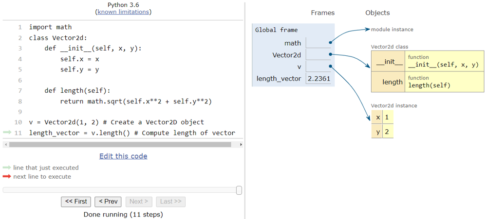
Figure 3. Vector2d class and object. (Click image for full-size view.)
Stepping through the code in Python Tutor shows that Python performs the following actions when the corresponding line of code is executed:
- Line 1 creates a module object (on the heap) and assigns it to the variable math (on the stack).
- Line 2 creates an object (on the heap) to represent the Vector2d class and assigns it to the variable Vector2d.
- Line 10 creates a Vector2d object and assigns it to the variable v.
- Line 11 computes the length of the Vector2d object and assigns it to the variable length_vector.
For user-defined classes, Python Tutor shows the methods defined inside a class as well as the individual data attributes inside an object. Here, it shows that:
- The Vector2d class has two methods __init__ and length.
- The Vector2d object has two data attributes x and y with values of 1 and 2, respectively.
3.3.2.3 Mutability, Aliasing, and Copying
The Vector2d objects are mutable. After you create a Vector2d object, you can change its data attributes using attribute assignment statements. These are assignment statements that contain a data attribute on the left:
In [8]: w = Vector2d(0, 0)  # Create null vector

In [9]: w.x, w.y
Out[9]: (0, 0)

In [10]: # Create unit vector in x-direction

In [11]: w.x = 1  # Attribute assignment

In [12]: w.x, w.y
Out[12]: (1, 0)
Here, you used an attribute assignment to update the x data attribute of w.
Similar to built-in objects, binding an existing Vector2d object to a new variable using assignment does not create a new Vector2d object. Python creates an alias. For example:
In [13]: u = Vector2d(0, 0)  # Creates a new Vector2d object and assigns to u

In [14]: v = u               # Creates a new variable and assigns id of u to v
Now, both u and v refer to the same Vector2d object as can be seen in the following Python Tutor visualization.
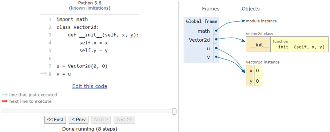
Figure 4. Aliased Vector2d objects. (Click image for full-size view.)
Now, you can update the data attributes of the object using v:
In [15]: v.y = 1   # Update y data-attribute of v

In [16]: u.x, u.y  # The y data-attribute of u is also updated
Out[16]: (0, 1)
You can make copies of objects (created from user-defined classes) by using the copy function in the copy module:
In [17]: import copy

In [18]: u = Vector2d(0, 0)

In [19]: v = copy.copy(u)  # Create a new Vector2d object by copying u

In [20]: v.y = 1           # Update y data-attribute of v

In [21]: u.y               # The y data-attribute of u is not updated
Out[21]: 0
Updating v does not update u since u and v are different objects:
In [22]: u is v
Out[22]: False
Copyright © 2022 Synopsys, Inc. All rights reserved.