
Sentaurus Topography 3D
7. Create and Use Masks From Layout Files
7.1 Overview
7.2 Importing a Layout File (GDSII or OASIS)
7.3 Creating a Mask From a Layer
7.4 Mask Operations
7.5 Sidewall Profiles
Objectives
- To import a layout file (GDSII or OASIS) into Sentaurus Topography 3D.
- To create masks from imported layout layers and to pattern materials with them.
7.1 Overview
This section presents the standard steps needed to import a layout file, in GDSII or OASIS format, and to use this file to create masks for patterning materials in Sentaurus Topography 3D.
The complete project can be investigated from within Sentaurus Workbench in the directory Applications_Library/GettingStarted/sptopo3d/layout. If you are not familiar with Sentaurus Workbench projects, the preprocessed script file layout_t3d.cmd can be found in this directory.
To download the preprocessed script file, right-click the following link and choose Save Target As: layout_t3d.cmd.
To execute the file in Sentaurus Topography 3D on the command line, enter:
> sptopo3d layout_t3d.cmd
After the command file is executed, the generated TDR file is layout_t3d.tdr.
7.2 Importing a Layout File (GDSII or OASIS)
This section shows how to import a specific cell from a layout file (GDSII or OASIS), how to define a domain (clip) of the layout to be used, and how to specify the layers of the layout that need to be available for the creation of masks in Sentaurus Topography 3D.
The command define_layout is used to import a GDSII file (file name with suffix .gds) or an OASIS file (file name with suffix .oas). The file name is selected with the layout_file parameter:
define_layout name= $layout_name layout_file= "layout.oas" \
  layer_numbers= {41:0 46:0 47:0 48:0 50:0 52:0 54:0}\
  layer_names= {layer1 layer2 layer3 layer4 layer5 layer6 layer7}\
  cell= $cell\
  domain= $domain domain_min= {-2.300 -1.500} domain_max= {2.200 2.000} \
  scale= 1.0 shift_to_origin= @shift_to_origin@
The following keywords are mandatory for the complete definition of the layout:
- name sets the name of the defined layout to be used within Sentaurus Topography 3D.
- layout_file sets the name of a GDSII or an OASIS file from which the layout is read.
- layer_numbers sets a list of layer numbers that are read from a GDSII or an OASIS layout file.
- layer_names sets a list of layer names to be used instead of the layer numbers specified in the layer_numbers parameter. The number of entries in both lists must be the same.
- cell sets the name of the layout cell from which a domain is extracted.
- domain sets the name to be given to the domain that is extracted from a GDSII or an OASIS layout file.
- domain_max sets the coordinate of the maximum point of the layout domain in the layout coordinate system.
- domain_min sets the coordinate of the minimum point of the layout domain in the layout coordinate system.
The imported layout can also be scaled with the parameter scale (default: 1.0).
The parameter shift_to_origin helps to align the defined layout domain (see Clip1 in Figure 1) to the actual simulation domain. By default, it is set to true, which means that the lower-left corner of the layout domain will coincide with the origin (0,0) of the xy plane of the simulation domain (see Figure 2).
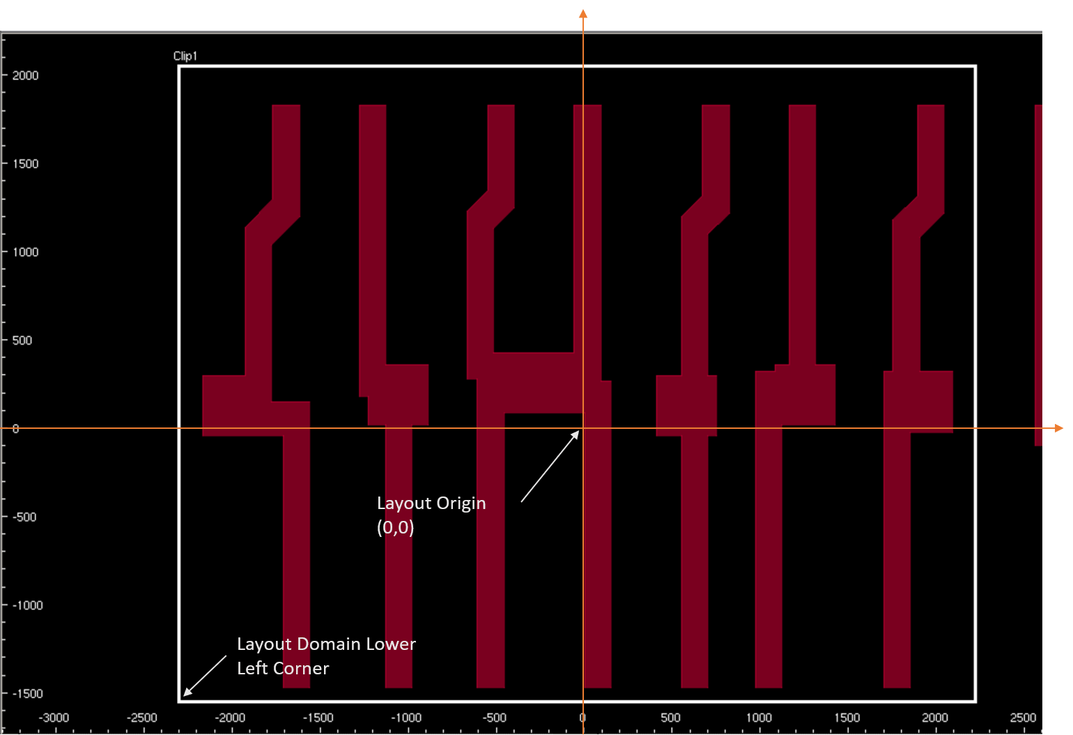
Figure 1. Plane view of the defined layout domain (highlighted with white box, named Clip1). The origin of the layout and the lower-left corner point of the layout domain are indicated. (Click image for full-size view.)
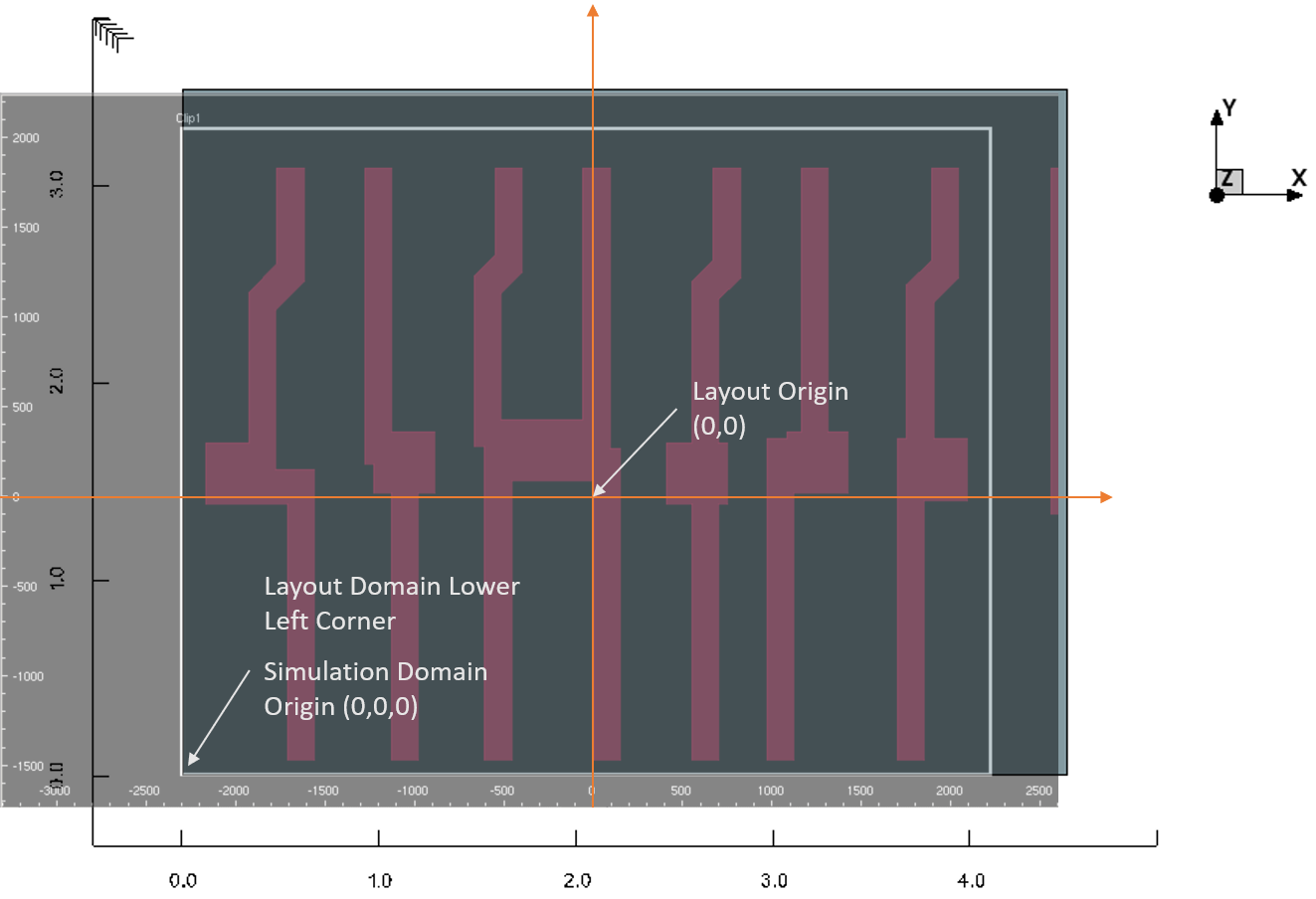
Figure 2. Overlay view of layout and simulation domains when shift_to_origin=true (default). In that case, the lower-left corner of the layout and the origin of the simulation domain (0,0,0) coincide. (Click image for full-size view.)
If shift_to_origin=false, then the origin (0,0) of the layout domain will coincide with the origin (0,0) of the xy plane of the simulation domain (see Figure 3). In the latter case, if the layout domain (clip) is defined far from the origin of the layout, then the result of the patterning with the masks defined from the layout might contain only some features (see Figure 4), or even none of them, if the clip lies completely outside of the simulation domain.
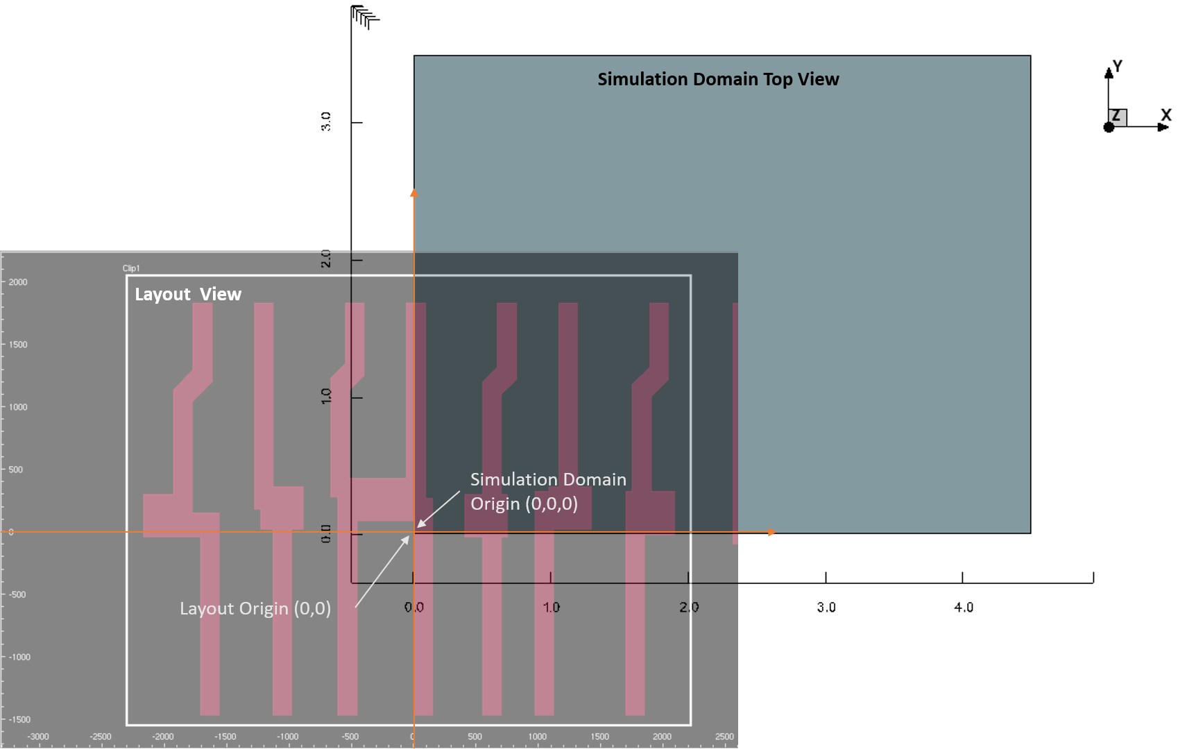
Figure 3. Overlay view of layout and simulation domains when shift_to_origin=false. In that case, the origin (0,0) of the layout and the origin of the simulation domain (0,0,0) coincide. (Click image for full-size view.)
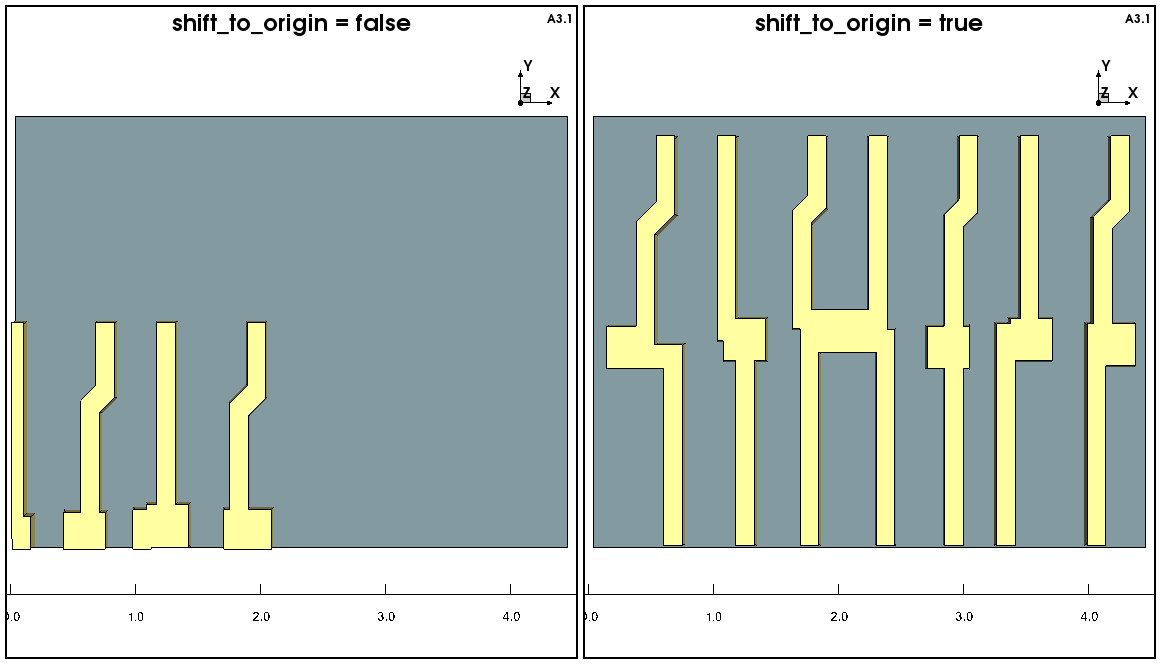
Figure 4. Top view of patterned photoresist when (left) shift_to_origin=false and (right) shift_to_origin=true. For shift_to_origin=false, the features available in the layout domain partially cover the simulation domain. No features are available for patterning outside the defined layout domain, Clip1. If shift_to_origin=true, then all features in the defined layout domain are available for patterning in the simulation space. (Click image for full-size view.)
7.3 Creating a Mask From a Layer
This section presents how to define a mask from a layer that is imported from a layout in the previous step. The command define_mask is used for this purpose with parameters for the complete definition of the mask:
define_mask name= mask_${layer1}_${domain} \
  layout= $layout_name domain= $domain layer= $layer1
The name of the mask defined with the parameter name must be unique. The parameters layout, domain, and layer refer to the already defined layout, the layout domain, and the layer, respectively, with the define_layout command.
7.3.1 About Masks, Reticles, and Photoresist Types
The masks that are created in Sentaurus Topography 3D are sets of geometric shapes (polygons) that can be used to pattern materials in the structure, and they do not have a polarity. The types of reticle (based on the defined mask) and types of photoresist assumed are defined at the patterning phase with the pattern or etch command, and there are four combinations of reticle and photoresist types: light_positive, light_negative, dark_positive, and dark_negative.
A reticle has one of two types depending on whether the mask areas covered by polygons transmit or block light:
- When exposing a reticle of type dark field, light is transmitted in areas that lie inside of the layout polygons, and light is blocked in areas that lie outside of the layout polygons.
- When exposing a reticle of type light field, light is transmitted in areas that lie outside of the layout polygons, and light is blocked in areas that lie inside of the layout polygons.
Similar to reticles, there are different types of photoresist:
- When exposed and developed, a negative photoresist is removed from areas that were not exposed to light, and it remains in areas that were exposed to light.
- When exposed and developed, a positive photoresist is removed from areas that were exposed to light, and it remains in areas that were not exposed to light.
Although there are four different combinations of reticle and photoresist types, there are only two possibilities for how material is deposited, as follows:
- Material is deposited in areas where the polygons are located in the logical mask (dark_negative and light_positive).
- Material is deposited in areas that are not covered by polygons in the logical mask (dark_positive and light_negative).
When considering the resulting region from a patterning operation, it is redundant to provide all four combinations. Nevertheless, providing all combinations makes it possible to specify the intended process explicitly.
7.3.2 Patterning Materials Using Masks
The defined masks can be used to pattern materials by using either an additive approach with the pattern command or a subtractive approach with the etch command. For example, the mask in Figure 2 could be used to pattern directly an aluminum layer (see Figure 5) as follows:
pattern material=Aluminium thickness=0.5 mask= mask_layer1_Clip1 \
  type= light_positive
The reticle type is defined in the pattern command and can be one of the types discussed in Section 7.3.1 About Masks, Reticles, and Photoresist Types. The sidewall profile from this etch is vertical, corresponding to a perfectly anisotropic etching.
It would have been possible to use the etch command instead of the pattern command to produce the plot in Figure 5. An additional step would also be needed to deposit the aluminum layer first by using the fill command as follows:
fill material=Aluminum thickness=0.5
etch thickness=0.5 mask= mask_layer1_Clip1 type= light_positive
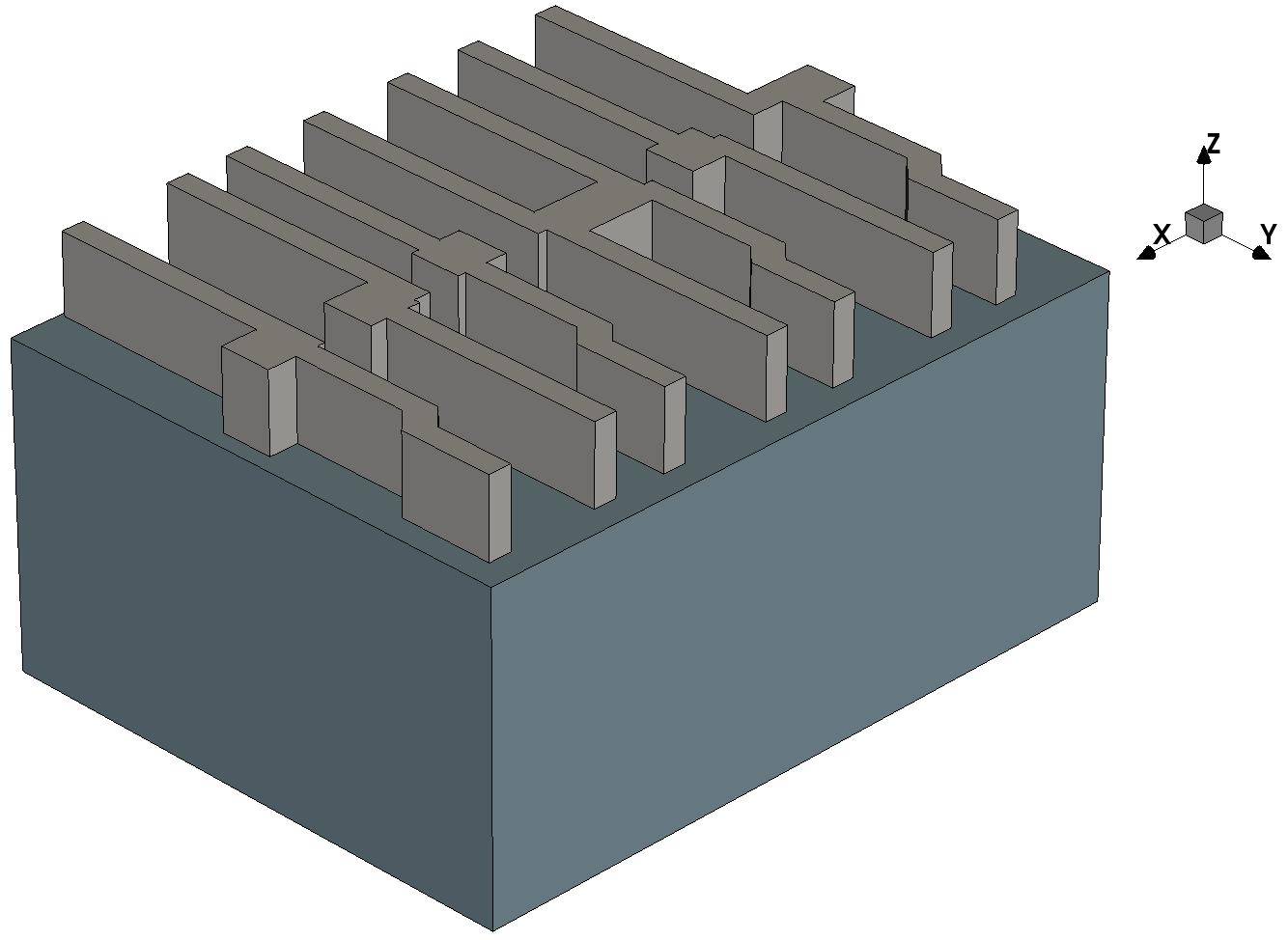
Figure 5. Patterned aluminum using the mask configuration shown in Figure 2. (Click image for full-size view.)
7.4 Mask Operations
Previously defined masks can be combined in pairs with binary operations.
This section presents the different ways that two masks can be combined to generate new masks. Masks that are derived from binary operations can themselves be used in new operations with other masks.
The binary operations that are used to form a new mask can be interpreted as set operations (difference, intersection, symmetric_difference, or union) on the polygons in the masks. Except for difference, these operations can also be interpreted as simple Boolean operations (not, and, xor, or or) where areas covered by polygons have the value true, and areas that are not covered by polygons have the value false.
To combine two masks with an operation, the command define_mask is used as follows:
define_mask name= Mask_Operation operation= @operation@  \
  mask1= "Mask_1" mask2= "Mask_2"
The Sentaurus Workbench parameter @operation@, for the mask operation between Mask_1 and Mask_2, can take one of the following values:
- difference
- intersection
- symmetric_difference
- union
It is important to note that, for the difference and symmetric_difference operations, the order in which masks are defined with the parameters mask1 and mask2 plays a role in the final result as the difference operation is mask1 – mask2.
Figure 6 shows the result of the mask operations with the help of the top views of patterned materials. The result of patterning aluminum with Mask_1 is the upper-left plot. Copper is patterned only with Mask_2. The other plots show the patterning of tungsten with the four different combinations of Mask_1 with Mask_2 by using the difference, intersection, symmetric_difference, and union mask operations.
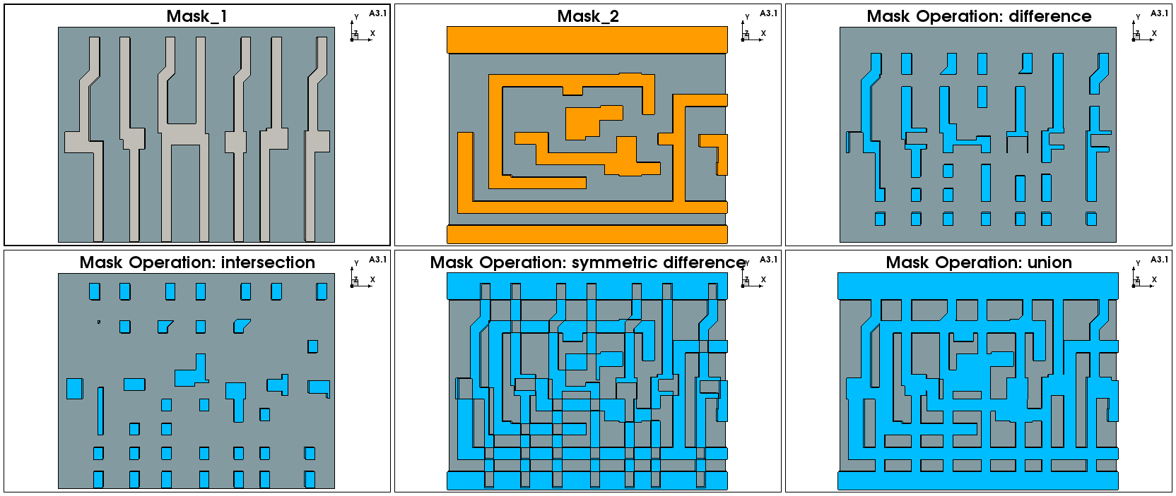
Figure 6. Mask operations between two masks, Mask 1 and Mask 2. Plots are top views of patterned materials. Patterning an aluminum layer with Mask 1 produces the upper-left plot (gray-colored material). Copper is patterned with Mask 2. Tungsten (blue-colored material) is patterned with various combinations of Mask1 and Mask 2 using the difference, intersection, symmetric_difference, and union mask operations. (Click image for full-size view.)
The operation complement is reserved for a single mask. As its name suggests, this operation generates a new mask where the polygon area coverage is inverted, that is, areas that were previously not covered by polygons are now covered, and vice versa. The syntax to create the complement of an existing mask is as follows:
define_mask name= CMask operation= complement mask1= Mask
7.5 Sidewall Profiles
Often when a layer needs to be patterned, it is critical to accurately reproduce the shape of the layer's sidewalls after this patterning step, as it could affect the geometry of the generated features in subsequent steps. In Sentaurus Topography 3D, you can create patterned layers as shapes that have a particular sidewall profile.
This functionality is demonstrated on the geometry of structure S4 in the Sentaurus Workbench project mentioned in Section 7.1 Overview. The define_shape command with the deposit command generate a patterned shape with a mask with a specific sidewall profile as follows:
define_shape name=shape1 type=mask reticle_resist_type=@reticle_type@  \
  profile= {0.0 2.5 -0.02 2.25 +0.01 2.1 -0.01 2.0} \
  mask=mask_${layer1}_${domain}

deposit material=Photoresist shape=shape1 structure= S4
The parameter reticle_resist_type can take the following values defined by the Sentaurus Workbench parameter @reticle_type@: light_positive, light_negative, dark_positive, and dark_negative.
The sidewall profile is defined with the parameter profile and a list of values in pairs. The first value in the pair is the offset length in micrometers of the sidewall at the specified z-coordinate, which is the second value in the pair. The offset length is the distance of the sidewall surface point at the specified z-coordinate from the plane formed by a virtual perfectly vertical sidewall at the mask edge.
If the offset length is negative, then the sidewall is retracted with respect to the vertical sidewall plane. The opposite occurs when the offset length is positive, creating an overhang of the sidewall at that point. A linear interpolation is used to define the sidewall profile between two z-coordinate points in the profile list.
At the top of the photoresist (z-coordinate is 2.5 μm), the offset length is 0.0. At Z=2.25 μm, the sidewalls are retracted by 20 nm and, at Z=2.1 μm, the sidewalls have an overhang of 10 nm. Finally, at the bottom of the photoresist, the sidewalls are again retracted by 10 nm.
Figure 7 shows the cross section of the patterned photoresist profile with the corresponding profile pairs. Figure 8 shows the resulting photoresist structure.
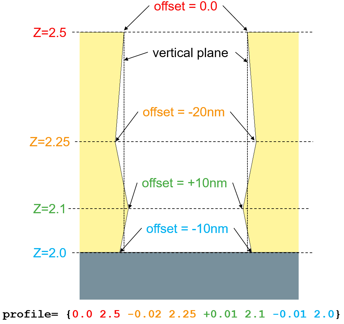
Figure 7. Cross section of patterned photoresist showing sidewall profile and corresponding values of the list defined with the profile parameter. (Click image for full-size view.)
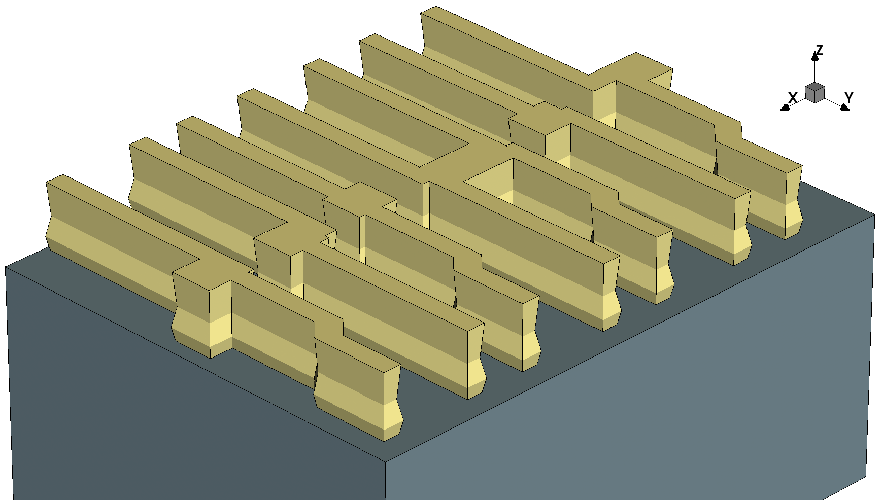
Figure 8. Patterning of a photoresist layer with a specific sidewall profile. The defined profile is applied to all sidewalls. (Click image for full-size view.)
The sidewall profile can also be defined by using the slope of the sidewalls between two specific z-coordinates using the taper_angles parameter. For example:
define_shape name=shape2 type=mask mask=mask2 \
  z_coordinates={3.0 2.5 2.0 1.5 1.0} taper_angles={ -10  15  0  -5 }
Here, the slope is –10° (retracting sidewall) between Z=3.0 μm and Z=2.5 μm, then 15° between Z=2.5 μm and Z=2.0 μm, and so on for the other values of z_coordinates and taper_angles. Note that the length of the taper_angles list is N – 1, where N is the length of the z_coordinates list.
Copyright © 2022 Synopsys, Inc. All rights reserved.