main menu | module menu | << previous section | next section >>

Sentaurus Topography 3D
8. Extract and Visualize Geometric and PMC Data

8.1 Overview
8.2 Create Extraction Boxes for Runtime PMC Data
8.3 Runtime Extraction of Surface-Mapped PMC Information
8.4 Postprocess Shape Analysis Extractions

Objectives

To extract geometric and surface reaction data from a PMC simulation.
To visualize the extracted quantities.

8.1 Overview

This section is dedicated to the extraction of crucial information (also called metrology in the text) from Sentaurus Topography 3D PMC simulations. This information can be extracted during the PMC simulation runtime or as postprocessing steps after the simulation is finished.

You can use Sentaurus Visual for visualization and further processing of the extracted data. A Sentaurus Workbench project (see Figure 1) is available with a complete example of an ion-assisted etch simulation (the same as in Section 6.3 Example: PMC Ion-Assisted Etching) and the associated metrology steps along with the Sentaurus Visual tool instances to facilitate visualization.

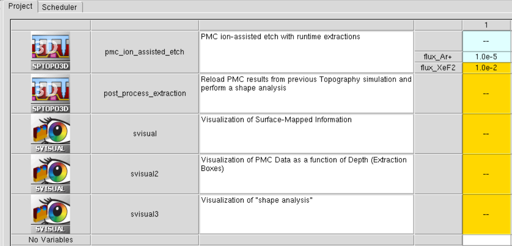
Figure 1. PMC metrology Sentaurus Workbench project in vertical layout. (Click image for full-size view.)

The first Sentaurus Topography 3D tool instance performs an ion-assisted etch (as in Section 6.3 Example: PMC Ion-Assisted Etching) and executes the runtime extractions to obtain critical PMC data. The second Sentaurus Topography 3D tool instance reads the .pmc restart file saved in the first tool instance and performs the shape analysis extraction to obtain the geometric characteristics of the etched feature.

Three Sentaurus Visual tool instances are included in the project to demonstrate how to load and visualize the CSV and TDR files generated in the first two Sentaurus Topography 3D tool instances. Comments are added to help you distinguish the functionality of each tool.

The complete project can be investigated from within Sentaurus Workbench in the directory Applications_Library/GettingStarted/sptopo3d/PMC_Metrology.

If you are not familiar with Sentaurus Workbench projects, then the preprocessed script files pp_pmc_ion_assisted_etch_t3d.cmd and pp_post_process_extraction_t3d.cmd can be found in this directory.

To download the preprocessed script files, right-click the following links and choose Save Target As:

To execute the PMC simulation file in Sentaurus Topography 3D on the command line, enter:

> sptopo3d pp_pmc_ion_assisted_etch_t3d.cmd

To run the PMC metrology file in Sentaurus Topography 3D on the command line, enter:

> sptopo3d pp_post_process_extraction.cmd

8.2 Create Extraction Boxes for Runtime PMC Data

You can extract information about the simulated structures during runtime by using the command define_extraction. This information covers the geometric characteristics of the simulated structure such as dimensions, material thicknesses (see also the example in Section 6.3 Example: PMC Ion-Assisted Etching), areas, volumes, feature profiles as well as the events occurring on the surface, for example, the impact of gas species, the reactions, or the reemission of particles.

In PMC simulations, you can select specific parts of the simulation domain using bounding boxes in order to extract the PMC data for the reactions occurring in the part of the PMC simulation domain contained within the boxes. It is also possible to perform an extraction on an axis-aligned 2D plane (normal to the x-, y-, or z-axis) by specifying the keywords axis and position in the command define_extraction. For example:

define_extraction type=pmc_data name=pmc_stats \
  quantities= {reaction_executions sputtered_volume sputter_yield} \
  axis=x position=0.1 reactions= {R1 R2 R3} \
  csv_file= pmc_data_box_2D_cut.csv

The extraction can be executed at user-defined time intervals during the PMC simulation defined with the keyword extraction_interval in the command etch. Multiple extraction boxes can be defined and grouped under the same name using the command define_extrusion and the keyword name.

Various quantities regarding the gas species, the surface reactions, and their products can be included in the extracted data:

deposited_volume: Volume of deposited species
reaction_executions: Number of reaction executions
species_volume: Total species volume in the PMC simulation domain
sputter_yield: Effective sputter yield for various gas species and surface materials (for the reactions to which this applies, that is, sputtering reactions)
sputtered_volume: Total volume of sputtered species
volumetric_source_particles: Density of emission points of volumetric source species in the extraction box

For models with many surface reactions, only a small set of reactions might be of interest, and they can be defined using a list with the keyword reactions or by specifying reaction name patterns with glob syntax by using the keyword expression_pattern. For example:

expression_pattern="*SiFx*"

The results of the PMC data extraction can be saved in a comma-separated file (with the .csv file extension) and visualized in Sentaurus Visual or in a spreadsheet application. In the Sentaurus Workbench project PMC_Metrology, two extraction boxes are defined (see Figure 2) with a for loop. The first extraction box covers the lower half of the structure and the second extraction box covers the upper half of the structure. In addition, an extraction definition on a 2D plane is added in the same group named pmc_stats.

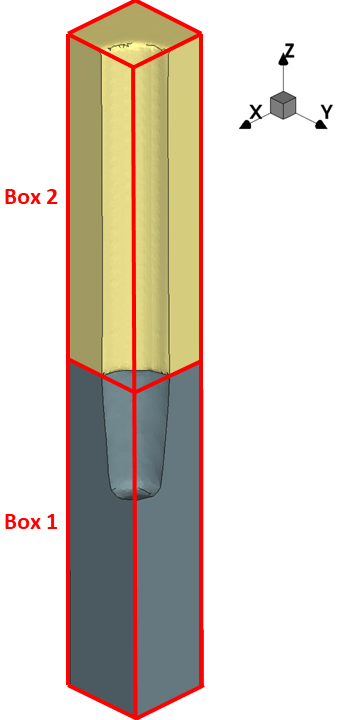
Figure 2. Extraction boxes location in the structure: Box 1 covers the lower half of the hole and Box 2 covers the upper half of the hole. (Click image for full-size view.)

The commands for the defined extractions are given here:

set number_of_boxes 2
for {set i 1} {$i <= $number_of_boxes} {incr i} {
    set step [expr $bbox_z_length/$number_of_boxes]

    ## Define extraction for PMC reactions' statistics for box No. $i 
    define_extraction type=pmc_data name=pmc_stats \
       quantities= $quantities  \
       reactions= {sput_Si refl_Si sput_SiFx refl_SiFx adsorb_F_Si etch_F_Si} \
       csv_file=n@node@_pmc_stats_box_${i}.csv \
       point_min= "$bbox_xmin $bbox_ymin [expr $bbox_zmin+($i-1)*$step]" \
       point_max= "$bbox_xmax $bbox_ymax [expr $bbox_zmin+($i)*$step]"
}

define_extraction type=pmc_data name=pmc_stats \
   quantities= $quantities axis=x position=[lindex $bbox_xmin 0] \
   reactions= {sput_Si refl_Si sput_SiFx refl_SiFx adsorb_F_Si etch_F_Si} \
   csv_file=n@node@_pmc_stats_box_2D_cut.csv

The results of the extractions are saved in the files named n@node@_pmc_stats_box_1.csv (for Box 1), csv_file=n@node@_pmc_stats_box_2.csv (for Box 2), and n@node@_pmc_stats_box_2D_cut.csv (for 2D cutplane). At every defined time interval with the keyword extraction_interval in the etch command, the extracted data is appended to those files as in the following example:

etch machine=rie_machine spacing=0.002 time=1000.0<s> method=pmc \
   extraction=pmc_stats extraction_interval= 250.0<s>\
   plot_type={surface} plot_interval=250.0<s> file=n@node@_surface.tdr

The extracted data can be visualized with Sentaurus Visual as demonstrated in the svisual1 tool instance as shown in Figure 3.

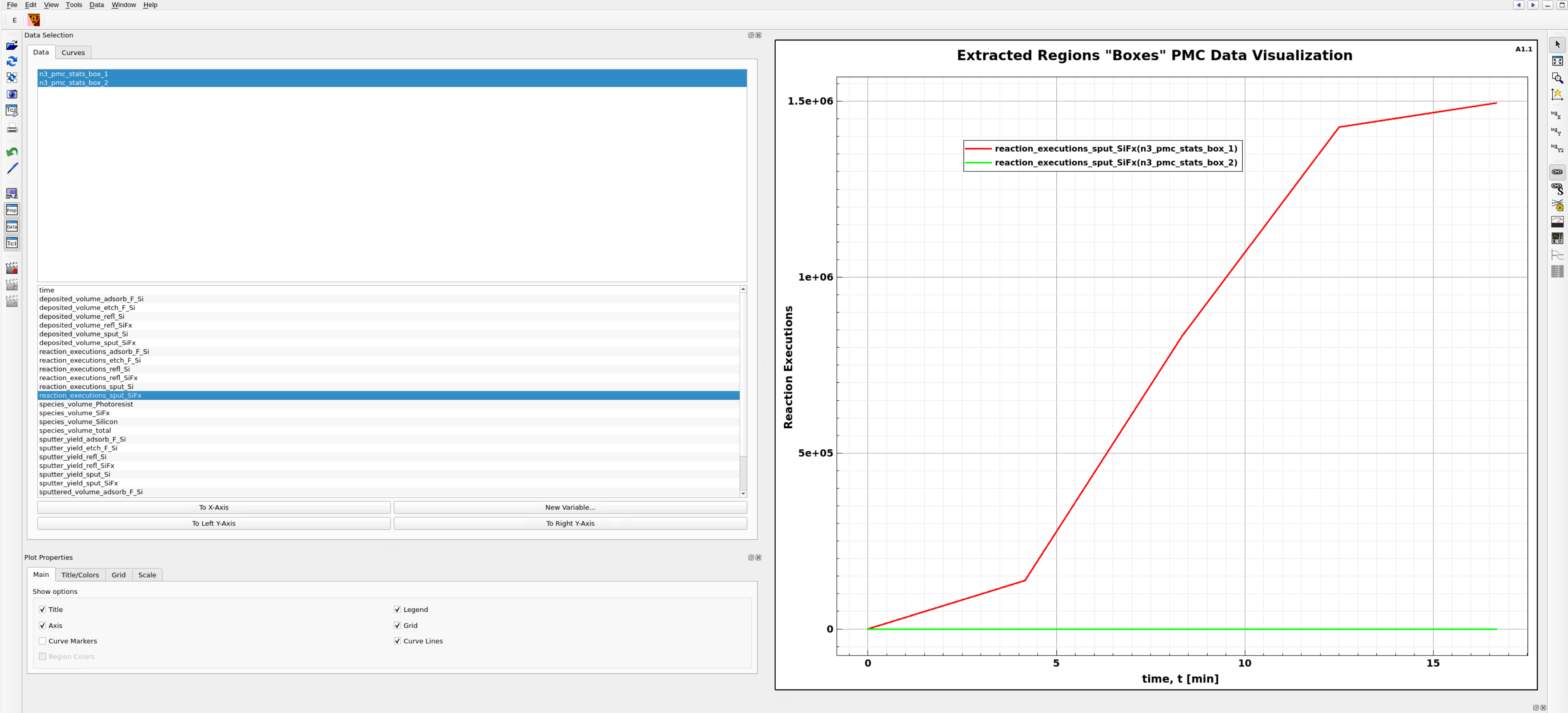
Figure 3. Screen capture of Sentaurus Visual showing the available data stored in the .csv files extracted at runtime of the ion-assisted etch PMC simulation. (Click image for full-size view.)

In Figure 3, the reaction executions for the sputtering reaction of SiFx are plotted as a function of time. In the upper part of the structure, only the photoresist mask is present, so there is no silicon or SiFx species and the executions are zero (green line). In the lower part (red line – Box 1) of the structure, sputtering is increased when Ar⁺ ions are introduced (see Figure 5 in Section 6.3.1 PMC Time-Dependent Species Distributions). The number of executions flattens out when the flux of XeF₂ is switched off and only the remaining SiFx is sputtered from the surface by Ar⁺ ions without any new SiFx being created.

More data about the reaction executions from the ion-assisted etching model can be visualized as a function of time as shown in Figure 3.

8.3 Runtime Extraction of Surface-Mapped PMC Information

In addition to the extraction of volume-averaged PMC data with boxes or 2D planes, you can extract PMC information mapped on to the exposed surface at user-defined intervals or specific time points during the simulation. You can do so by using the keywords plot_interval (or plot_times for a list of specific times) and plot_type.

The following supported plot types for PMC simulations are saved in a TDR file defined by the file parameter:

gc: GC type of TDR file.
surface: TDR file of the exposed surface at each time interval on which PMC information is mapped (reactions, fluxes, reemissions, reflections, and so on). The extracted surfaces are appended in the same TDR file (defined by the parameter file in the etch command) at each time interval.
vbe: Boundary representation saved in the TDR file directly extracted from the PMC domain.
volume_fractions: Grid-based species volume fractions saved in the TDR file.

An example of a surface plot saved during ion-assisted etching is given in the Sentaurus Workbench project PMC_Metrology, and it is visualized with the Sentaurus Visual tool instance named svisual2 (see Figure 4). The definition of plot_intervals is performed directly in the etch command:

etch machine=rie_machine spacing=0.002 time=1000.0<s> method=pmc \
   extraction=pmc_stats extraction_interval= 250.0<s>\
   plot_type={surface} plot_interval=250.0<s> file=n@node@_surface.tdr

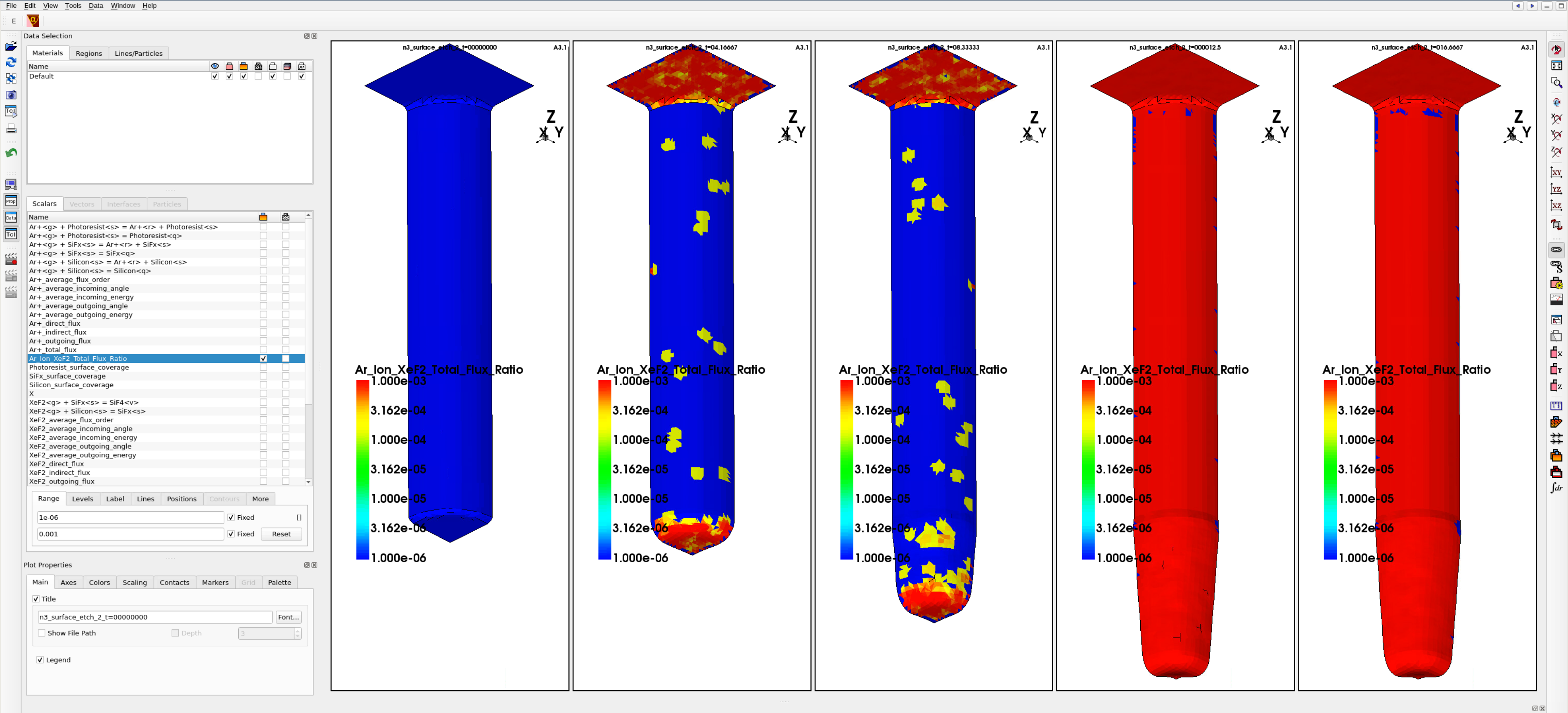
Figure 4. Surface mapping of flux ratio Ar⁺/XeF₂. In the beginning of the process, the Ar⁺ flux is zero. Later both fluxes, Ar⁺ and XeF₂, are switched on and the ratio increases on the horizontal surfaces but is much less on the sidewalls due to the high directionality of the Ar⁺ ions. At the end of the etching cycle, the flux of XeF₂ is switched off and the flux ratio Ar⁺/XeF₂ takes its maximum value on all surfaces. Many other fields are available for visualization as shown on the left side of the Sentaurus Visual window. (Click image for full-size view.)

8.4 Postprocess Shape Analysis Extractions

The Sentaurus Topography 3D tool instance labeled post_process_extraction loads the PMC restart file from the previous Sentaurus Topography 3D tool instance and performs a shape analysis of the etched feature in the structure.

To load the PMC restart file, specify the define_structure command with the parameter pmc_file as follows:

define_structure pmc_file=n@node|pmc_ion_assisted_etch@_result.pmc

The PMC file can only be used to restart the PMC simulation from the point at which it stopped in the previous step after the ion-assisted etching (it cannot be visualized with Sentaurus Visual). After the state of the PMC simulation is reestablished after loading the PMC file, it is possible to continue with another PMC simulation step or to use the extract command to extract metrology information. Here, the extract command is used as a postprocessing step to perform a shape analysis of the structure, which is a cylindrical hole etched in silicon. The command syntax is the following:

extract name=shape_analysis  type=shape_analysis \
   reference_shape=cylinder_hole max_radius=0.03 \
   point1="$bbox_middle_x $bbox_middle_y $bbox_zmin" \
   point2="$bbox_middle_x $bbox_middle_y $bbox_zmax" \
   csv_file=n@node@_shape_analysis.csv output_type={doe csv} smoothing_order=0

Two reference shapes can be used depending on the feature geometry: either cylinder_hole for structures with cylindrical symmetry or trench for structures that have a groove-like shape as a trench. The cylindrical bounding box is specified by two points (point1 and point2) that define the bottom and top of the vertical cylinder axis, and by the radius (max_radius) of the cylinder (see Figure 5).

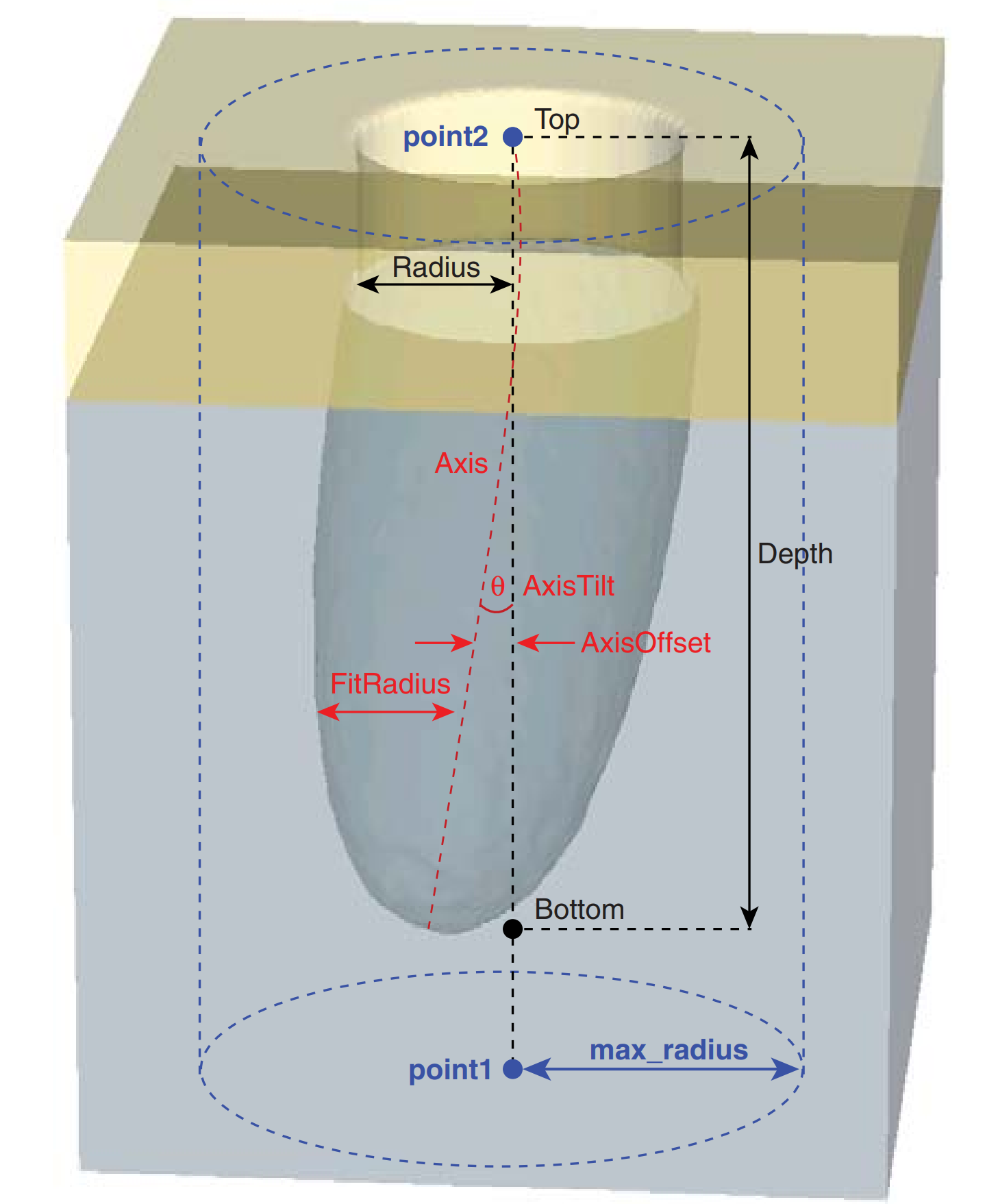
Figure 5. Definition of extraction window for shape analysis when reference_shape=cylinder_hole. (Click image for full-size view.)

The extracted metrics from the shape analysis can be saved in a CSV file (defined with the parameter csv_file), in a TDR file (defined with the parameter tdr_file), and also as Sentaurus Workbench variables by setting output_type={ csv tdr doe }. The doe option generates the variables that are shown automatically at the end of the extraction in the Sentaurus Workbench project (see Figure 6).

See the Sentaurus™ Topography 3D User Guide, Shape Analysis, for detailed explanations of these variables in the tables in that section.

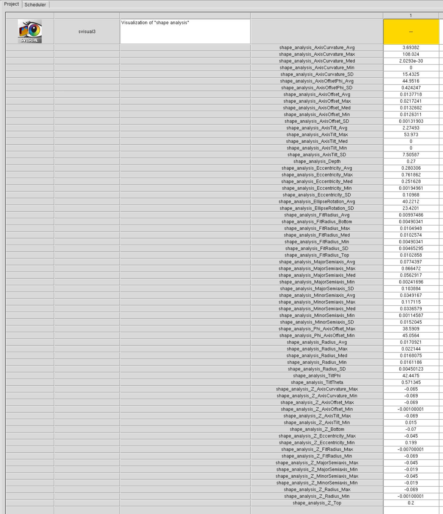
Figure 6. Shape analysis extracted metrics exported as Sentaurus Workbench variables. (Click image for full-size view.)

The CSV or TDR files containing the shape analysis information can be loaded in Sentaurus Visual to plot the extracted metrics as a function of depth Z as shown in Figure 7 and Figure 8. The same type of plot is generated by running the node of the Sentaurus Visual labeled svisual3 in the project PMC_Metrology.

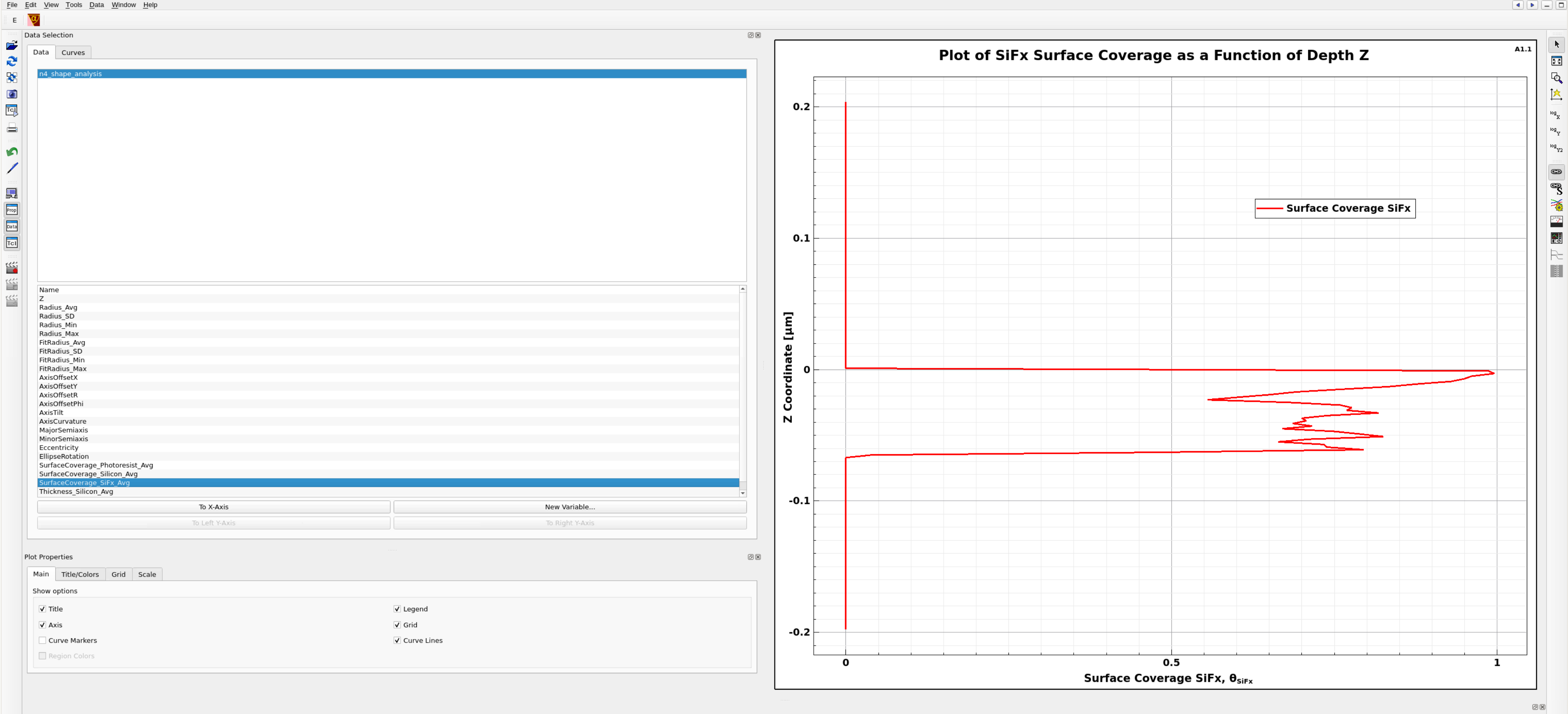
Figure 7. Plot generated by svisual3 Sentaurus Visual tool instance showing the average surface coverage of species SiFx as a function of depth in the cylindrical hole. The values are zero on the sidewalls of the photoresist mask for Z > 0 and for Z < -0.07 μm in bulk silicon. SiFx coverage on the sidewalls drops with depth as fluorine species have a higher probability (high reactivity) of reacting with silicon at the upper part of the hole and is also very low at the bottom where SiFx is heavily sputtered by Ar⁺ ions. A similar plot can be created by using the average radius of the hole, which will correspond to the hole profile (Figure 8). (Click image for full-size view.)

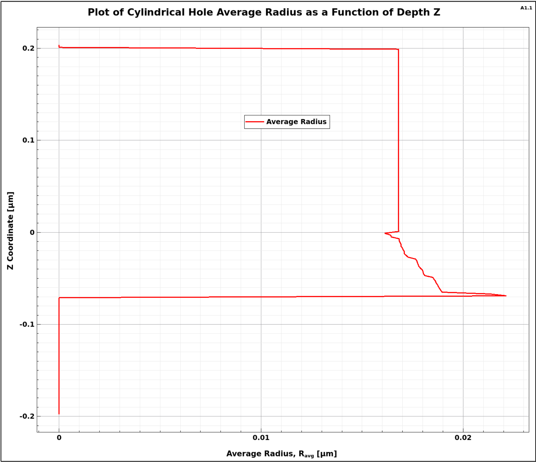
Figure 8. Plot of cylindrical hole average radius as a function of depth Z as extracted by shape analysis. (Click image for full-size view.)