
Sentaurus Topography 3D
5. Particle Monte Carlo Reaction Modeling
5.1 Introduction to the Particle Monte Carlo Engine
5.2 Defining the PMC Model
5.3 Defining the Source Species Characteristics
5.4 Defining the PMC Machine
5.5 Defining the PMC Model Reaction Properties
5.6 Running the PMC Simulation
Objectives
- To provide a basic understanding and setup of the particle Monte Carlo (PMC) reaction models in Sentaurus Topography 3D.
5.1 Introduction to the Particle Monte Carlo Engine
The PMC engine for feature-scale simulation of etching and deposition processes is based on a cellular grid representation of the wafer structure, and a PMC technique to model the fluxes of plasma-generated species to the wafer surface. Simulations with the PMC engine are always run in three dimensions. For the same model and similar accuracy, the PMC engine is, in general, significantly faster than the level-set engine, up to factors of 100 and more.
In contrast to the level-set engine, which calculates etching and deposition rates on the gas–material interface (as shown in Section 4. Working With the Rate Formula Module) and then advances this interface accordingly, the PMC engine relies on a set of user-specified surface reactions that control the interactions of plasma-generated species with the exposed part of the wafer representation.
This modeling approach is natural, versatile, and simple, because each surface reaction describes only one elementary interaction of the plasma-generated species with one of the species on the wafer surface.
5.1.1 Main Parts of a PMC Process Step
A PMC process step is divided into four main steps that must be specified in the correct order in the Tcl command file to be executed by Sentaurus Topography 3D:
- Define the PMC model (see Section 5.2 Defining the PMC Model).
- Define the source species characteristics (see Section 5.3 Defining the Source Species Characteristics).
- Define the PMC machine (see Section 5.4 Defining the PMC Machine).
- Define the PMC model reaction properties (see Section 5.5 Defining the PMC Model Reaction Properties).
5.2 Defining the PMC Model
In PMC, instead of using an analytic formula for the etching or deposition rate (as in the rate formula module (RFM)), a set of reactions is used to model the interaction of the incoming species in the gas phase (tag <g> is used from now on) with the materials on the surface (tagged with <s> from now on). As for RFM models, the definition of a new reaction model starts with the define_model command and ends with the finalize_model command.
5.2.1 Defining the Source Species
Before writing the reactions, you must define all the incoming species in the gas phase that will be used in the PMC reaction model. There is no limitation to the names or the number of the species to be used. Of course, you cannot define two separate gas species with the same name.
Unlike the definition of a level set–based model, there is no distinction between ion and neutral species when the source species are defined in the model. The properties of the gas species (flux, and angular and energy distributions) are defined after the model definition, so the same model can be used with different gas species properties, if needed.
To define a new gas species (for example, fluorine (F)) in a PMC model, you use the add_source_species command after the define_model command as follows:
define_model name=PMCModel1 description="Simple Etch Model"

add_source_species name=F model=PMCModel1
...

finalize_model model=PMCModel1
5.2.2 Defining the Surface Reactions
After all the gas species are defined, the next step is to define the surface reactions of the model, that is, all the reactions needed between the gas species and the materials on the surface of the structure.
There are several types of surface reaction in PMC depending on their products. The syntax of a surface reaction resembles the syntax of a real chemical reaction: reactants are on the left side and products are on the right side of the reaction. Only one-way reactions are supported and only two reactants can appear on the left-hand side of the reaction, with the species in the gas phase (tagged with <g>) always being one of the two.
Stoichiometric reactions and mass preservation are not supported for PMC surface reactions. The following list shows the basic set of surface reactions that are available in PMC and the corresponding syntax using the add_reaction command:
add_reaction model=demo  name=adsorption \
   expression="A<g> + Mat1<s> = Mat1A<s>"

add_reaction model=demo  name=reemission \
   expression="B<g> + Mat1<s> = Mat1<s> + B<g>"

add_reaction model=demo  name=reflection \
   expression="C<g> + Mat1<s> = Mat1<s> + C<r>"

add_reaction model=demo  name=simple_etch \
   expression="D<g> + Mat1<s> = Mat1<v>"

add_reaction model=demo  name=sputtering_tracked \
   expression="E<g> + Mat1<s> = Mat1<p>"

add_reaction model=demo  name=sputtering_untracked \
   expression="G<g> + Mat1<s> = Mat1<q>"

add_reaction model=demo  name=nucleation \
   expression="H<g> + Mat1<s> = Mat2<s> + Mat1<b>"

add_reaction model=demo  name=growth \
   expression="H<g> + Mat2<s> = Mat2<s> + Mat2<b>"
The arbitrary species A, B, C, D, E, G, and H are assumed to have been previously defined with the add_source_species command.
5.2.3 Types of Surface Reaction
In this section, the surface reaction types presented in Section 5.2.2 Defining the Surface Reactions are explained in more detail.
add_reaction model=demo  name=adsorption \
   expression="A<g> + Mat1<s> = Mat1A<s>"
The first reaction named adsorption is used to model the adsorption of species A on the surface of material Mat1. The product is a particle of a new material called Mat1A on the surface (tagged <s>) that replaces one particle of Mat1. The product can have any name, but Mat1A has been chosen to remember more easily that A was adsorbed on Mat1. The particle A consumed during this reaction is removed from the simulation.
add_reaction model=demo  name=reemission \
   expression="B<g> + Mat1<s> = Mat1<s> + B<g>"
The reaction named reemission is used to model the reemission of species B from the surface of material Mat1. The products are the same as the reactants because the surface is not modified and species B has been put back into the gas phase. Nevertheless, it is possible to write a reemission reaction with a modified material on the surface.
Species B are reemitted strictly isotropically from
the surface, even if the initial angular distribution from its source was not
isotropic.
This reaction (reemission) is the default reaction executed
by the PMC engine when the reactants on the left-hand side are used in other
reactions that finally do not happen (stochastic process) in a cell.
add_reaction model=demo  name=reflection \
   expression="C<g> + Mat1<s> = Mat1<s> + C<r>"
The third reaction called reflection is distinguished from the reemission reaction by the product C tagged with <r> instead of <g>.
In this case, species C is reflected specularly (incidence angle equals reflection angle) on the surface of Mat1. It is possible to adjust the angular distribution of the reflected species in the properties of the specific reaction as shown later.
add_reaction model=demo  name=simple_etch \
   expression="D<g> + Mat1<s> = Mat1<v>"
Regarding the reaction simple_etch, species D reacts with Mat1 to produce the volatile species Mat1 (tagged <v>). The volatile species can have a different name than the material on the surface. Particles D and Mat1 consumed during this reaction are removed from the simulation. This means that, in this reaction, one incident particle D removes one particle Mat1 from the surface.
add_reaction model=demo  name=sputtering_tracked \
   expression="E<g> + Mat1<s> = Mat1<p>"

add_reaction model=demo  name=sputtering_untracked \
   expression="G<g> + Mat1<s> = Mat1<q>"
In cases when an energetic particle (mainly ions) impacts the surface, its kinetic energy might be enough to remove more than one particle at the same time (high yield). Such a mechanism is sputtering. In order to model it, a separate type of reaction is introduced in PMC where you need to specify a yield function to let the simulator know how many particles can be removed by the incoming particle. The ejected particles from the surface go into the gas phase, and they can potentially react with the materials on the surface.
If you want the simulator to track those ejected particles, so as to use them in the left-hand side of other reactions, you must use a reaction like the one named sputtering_tracked, where the ejected species on the right-hand side (products) are tagged with <p>.
Tracking ejected particles requires a certain amount of additional memory and CPU resources. So, in cases where you do not need to use the sputtered species in the left-hand side of other reactions, you can save computational resources by using a reaction like sputtering_untracked, where the particles (tagged <q>) that are removed from the surface are not tracked.
In both cases of sputtering reactions, you must provide a yield function for the reaction using the define_yield command as shown in Section 4.2.3 Modeling a Neutral Flux and an Ion Flux With Sputtering. The yield function can be angle dependent and energy dependent, and can be customized by using an analytic formula as you will see later in the sputtering example.
add_reaction model=demo  name=nucleation \
   expression="H<g> + Mat1<s> = Mat2<s> + Mat1<b>"

add_reaction model=demo  name=growth \
   expression="H<g> + Mat2<s> = Mat2<s> + Mat2<b>"
So far, the reactions have as products either species that go to the gas phase or species that stay at the surface. The last reactions, nucleation and growth, introduce a new type of product tagged with <b>.
The particle of product species tagged with <b> is moved into the volume (bulk) of the structure and a particle of the product species tagged with <s> is added on top and becomes a new surface particle. In this way, material can be deposited on the surface.
The nucleation reaction is about adding, at the surface, a particle of a species that differs from the material that is already on the surface. The growth reaction is a deposition reaction that adds a particle of the same material as the existing material on the surface.
In general, for a deposition to proceed, both a nucleation reaction and a growth reaction are needed. If only a nucleation reaction is present, a monolayer of the material will be deposited, unless the deposited material is the same as the existing material on the surface. In both reactions, nucleation and growth, the reacting particle in the gas phase (precursor, <g> tag) is removed from the simulation after the reaction happens.
5.2.4 Finalizing the Model
After you have introduced all the source species and the necessary surface reactions, your model is ready to be finalized and used. As for RFM models, the command finalize_model must be added at the end of all source species and reaction additions to close the definition of a PMC model. The following example shows a complete model definition for etching:
define_model name=Si_F_Etch description="Etching Si with Fluorine"
add_source_species name=F model=Si_F_Etch

add_reaction name=adsorb_F_Si model=Si_F_Etch \
  expression="F<g> + Silicon<s> = SiF<s>"

add_reaction name=adsorb_F_SiF model=Si_F_Etch \
  expression="F<g> + SiF<s> = SiF2<s>"

add_reaction name=adsorb_F_SiF2 model=Si_F_Etch \
  expression="F<g> + SiF2<s> = SiF3<s>"

add_reaction name=etch_F_SiF3 model=Si_F_Etch \
  expression="F<g> + SiF3<s> = SiF4<v>"

finalize_model name=Si_F_Etch
5.3 Defining the Source Species Characteristics
PMC model definitions contain all the source species used by the models, but their properties (such as fluxes, angular and energy distribution functions, and yields) are not yet defined.
5.3.1 Defining the Source Species Distribution
To define the distribution function of a species and its flux, you use the command define_species_distribution. For example:
define_species_distribution name=distribution species=A exponent=1 flux=1.0e-3
define_species_distribution name=distribution species=B exponent=10 flux=1.0e-4
define_species_distribution name=distribution species=C exponent=100 \
  flux=3.4e-5 energy_min=5 energy_max=100
The keyword exponent defines the angular distribution of the species based on the formula cosm(θ) (as discussed in Section 2.3.1 Defining the Deposition Model). In contrast to level-set models, in PMC, the fluxes of source species are not normalized, but they are defined in absolute values with the keyword flux ([mol s-1m-2]).
As you can observe, the distributions of species A, B, and C share the same name. This means that they are grouped in the same collection of distribution functions (name=distribution) and, whenever this collection is called, all the source species distributions defined in it can be used. The distributions of all the source species used in a specific PMC model should be grouped together under the same name.
Note that, in the distribution collection defined before named distribution, there are species that are energy independent (A and B) as well as species that are energy dependent (C). Although this is allowed, you cannot use A, B, and C in the same PMC model. The species used in a PMC model can be either energy dependent or energy independent.
It is possible to visualize the defined distributions using the save command. Plots are saved in a TDR file and can be viewed with Sentaurus Visual. All the distributions in the collection will be saved in the TDR file. For example:
save species_distribution=distribution file=distr_functions.tdr
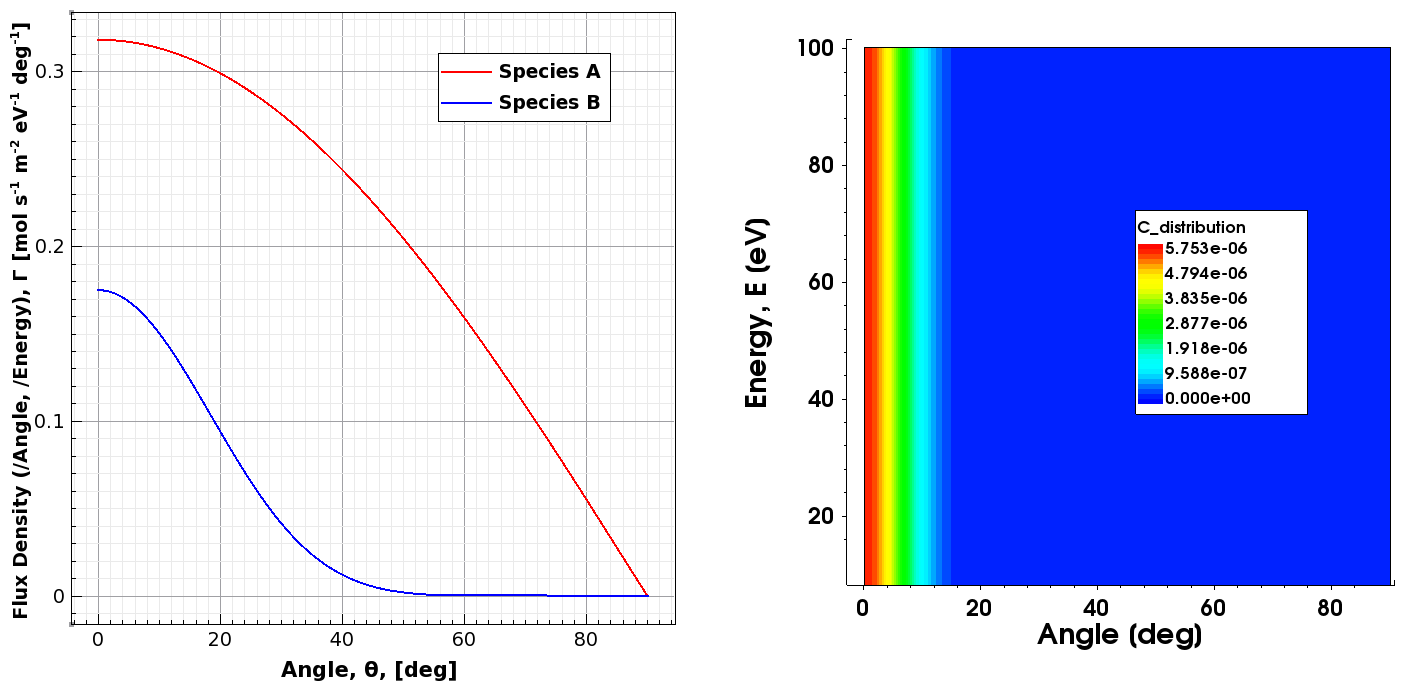
Figure 1. (Left) Plots of the distributions of species A and B, and (right) 2D contour plot of the energy-dependent distribution of species C. (Click image for full-size view.)
5.3.2 Energy Dependency of the Species Distribution Function
The distribution functions for species A and B do not contain any energy statement, which means the A and B particles emitted from the source do not carry any energy information – they are energy independent. On the other hand, the distribution for species C contains the keywords energy_min and energy_max (uniform distribution between the two values), which renders it energy dependent.
The distribution definitions for all species used in a PMC model are allowed to be either energy dependent or energy independent. You cannot mix energy-dependent and energy-independent source species in the same PMC model. So, depending on the distributions of the source species used in a PMC model, the latter can be characterized as either an energy-dependent or an energy-independent PMC model.
5.3.3 Defining the Source Species Material Yield Function
Whenever a sputtering reaction is present in a PMC model, it is mandatory to provide a yield function for it. The yield function is defined in the same way as for an RFM model (see Section 4.2.3 Modeling a Neutral Flux and an Ion Flux With Sputtering). The sputtering example in Section 5.2.3 Types of Surface Reaction used species E and G in sputtering reactions. For those species, it is necessary to define yield functions. For example:
define_yield name=yield species=E material=Mat1 \
  energy=0 yield_max=1.5 theta_max=54 yield_at_zero=1.0

define_yield name=yield species=G material=Mat1 \
  expression="max(0,((3.0*(sqrt(E)-sqrt(50.0)))*(1.0 - pow(sin(theta),10))))"
The defined yield for species G when it reacts with Mat1 uses an expression that is energy dependent (square root of E). This means that species G is part of an energy-dependent PMC model. Nevertheless, it is possible to use an energy-independent yield function even if the associated species is part of an energy-dependent PMC model, but not the other way around (that is, you cannot use an energy-dependent yield function for a species that is part of an energy-independent PMC model).
As this is the case for the source species distributions, yield definitions can be grouped in one yield collection by attributing the same name to all the yield definitions that belong to the collection.
As for the species distributions, it is possible to visualize the defined yields by using the save command. Plots are saved in a TDR file and can be viewed with Sentaurus Visual. All the yields in the collection will be saved in the TDR file. For example:
save yield=yield file=yield_functions.tdr energy_min=0 energy_max=100
When a collection for yield functions contains elements that are energy dependent, you must use the keywords energy_min and energy_max to produce 2D contour plots of the yield functions.
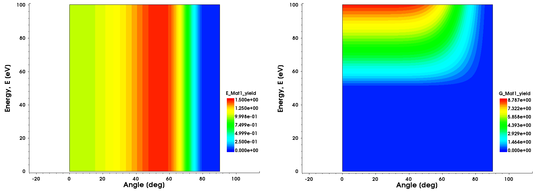
Figure 2. Two-dimensional contour plots of the yield functions of (left) species E and (right) species G. The yield function of species G is energy dependent. (Click image for full-size view.)
5.3.4 Defining the Source Species Properties: Default Event
As previously shown in the reemission reaction, this type of reaction (reemission) occurs by default (no need to explicitly add it in the model) if the main reaction between the specified reactants does not occur.
Each reaction of a PMC model has a probability to happen and you will see later how to define this probability. If the defined probability for a reaction is < 1, there is the likelihood that this reaction does not occur. In that case, the event, by default, is the reemission of the gas species from the surface at the point of incidence, which happens with an isotropic angular distribution.
You can change the behavior for the default event and discard the incoming gas particle instead of reemitting it with the following command:
define_species_properties default_event=discard name=properties species=C
Discarding the non-reacting gas particle means that it is removed from the simulation and it cannot react further with any surface material. Changing the default event is useful when you want to preserve the anisotropic characteristics of a species. If a gas species with a narrow angular distribution (high exponent value) does not react at a surface site and it is reemitted isotropically, then it starts to lose its anisotropic characteristics, and this behavior can lead to unexpected effects such as an increase in lateral etching. Figure 3 shows an exaggerated example of this parasitic effect.
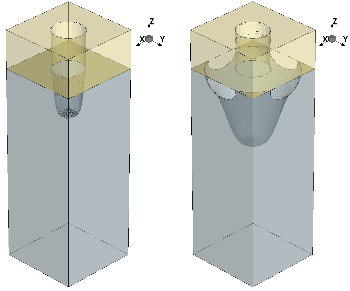
Figure 3. Default event effect on etching: (left) default event has changed to discard and (right) default event has retained its default value, that is, reemit. The effect on the shape is dramatic because the anisotropic species used for etching lose their highly directional character when default_event=reemit as they are reemitted isotropically from the surface. (Click image for full-size view.)
The properties of multiple species can also be part of a collection if they are defined with the same name, as is the case for the distributions and yield functions.
5.4 Defining the PMC Machine
The third step in the PMC process setup is the definition of a machine, which assembles the defined PMC model with the source species characteristics. In the following example, the fluorine PMC etching model of silicon is used to show the assembly in the machine with the fluorine distribution:
define_model name=Si_F_Etch description="Etching Si with Fluorine"
add_source_species name=F model=Si_F_Etch

add_reaction name=adsorb_F_Si model=Si_F_Etch \
   expression="F<g> + Silicon<s> = SiF<s>"

add_reaction name=adsorb_F_SiF model=Si_F_Etch \
   expression="F<g> + SiF<s> = SiF2<s>"

add_reaction name=adsorb_F_SiF2 model=Si_F_Etch \
   expression="F<g> + SiF2<s> = SiF3<s>"

add_reaction name=etch_F_SiF3 model=Si_F_Etch \
   expression="F<g> + SiF3<s> = SiF4<v>"

finalize_model name=Si_F_Etch

define_species_distribution name=distr species=F flux=1.0e-3 exponent=1 energy=0

define_etch_machine name=F_etch_machine model=Si_F_Etch \
   species_distribution=distr
In PMC, only the define_etch_machine command is used to define a machine even if the PMC model contains deposition reactions; this is the convention.
5.5 Defining the PMC Model Reaction Properties
The last step in the configuration of a PMC process is the addition of the properties of the surface reactions of the PMC model used in the machine. The properties are basically the probabilities of the surface reactions that are defined in the PMC model, which is used in the machine.
In the example of surface reactions used in Section 5.4 Defining the PMC Machine, you have four reactions that need to have their probabilities defined. For this purpose, you use the add_reaction_properties command for each reaction of the PMC model. For example:
add_reaction_properties machine=F_etch_machine reaction=adsorb_F_Si p=0.7
add_reaction_properties machine=F_etch_machine reaction=adsorb_F_SiF p=0.5
add_reaction_properties machine=F_etch_machine reaction=adsorb_F_SiF2 p=0.5
add_reaction_properties machine=F_etch_machine reaction=adsorb_F_SiF3 p=0.005
Notice that both the machine name and the reaction name must be defined. This means that the properties of the reactions might differ for different machines. The keyword p defines the probability as a number between 0 and 1.
It is possible to use an analytic expression for the probability of a reaction that can depend on the incidence angle or the energy of the incident particle. To do that, you need to predefine the analytic expression for the probability using the define_probability command before using it in the add_reaction_properties command. For example, you could write:
define_probability name=adsorb_F_Si_prob expression="0.7*cos(theta)"

add_reaction_properties machine=F_etch_machine reaction=adsorb_F_Si \
  probability=adsorb_F_Si_prob
Note the difference in usage between the keywords p and probability in the add_reaction_properties command. The keyword p is used to assign a number between 0 and 1; whereas, the keyword probability is used to call a probability expression that has been predefined with the define_probability command.
The probabilities that are defined with a mathematical expression using the define_probability command can also be saved in a TDR file for visualization. For example:
save probability=adsorb_F_Si_prob file=n@node@_probability.tdr
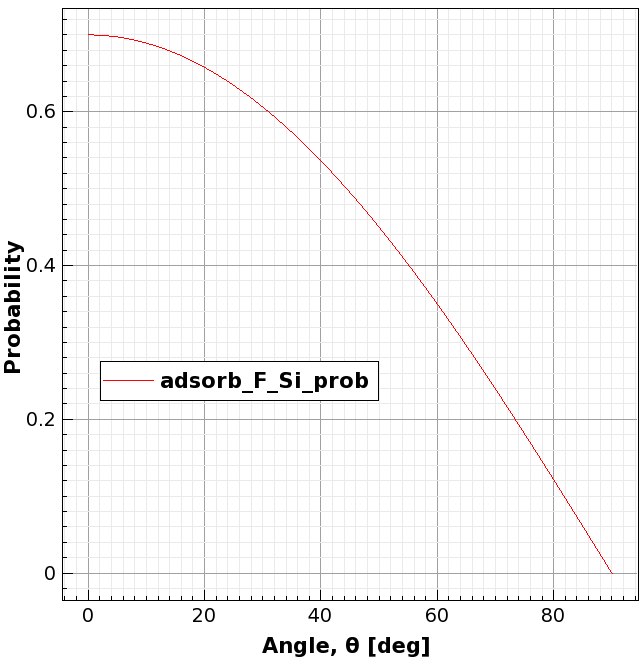
Figure 4. Plot of the defined probability adsorb_F_Si_prob. (Click image for full-size view.)
For PMC models that contain more than one reaction with the same pair of reactants on the left-hand side, the sum of the probabilities of all those reactions with a common pair of reactants must not exceed unity. This is also valid for probabilities defined by mathematical expressions, meaning that the condition for the sum of probabilities ≤ 1 must hold for all possible values of those expressions. Otherwise, an error is issued during runtime and the simulation stops.
If you have a reflection reaction, you can adjust the angular distribution (like a beam spreading) around the reflection (specular) direction. For example, assume you have defined the reflection reaction as before:
add_reaction model=demo  name=reflection \
   expression="C<g> + Mat1<s> = Mat1<s> + C<r>"
Then, the properties of this reaction can be set as follows:
add_reaction_properties machine=demo_machine reaction=reflection \
   reflection_exponent=10 p=0.1
If the reflection_exponent is omitted, then all the particles are reflected along the specular direction without any spreading. The smaller the reflection_exponent, the broader the spreading of the reflected particles around the specular direction.
5.6 Running the PMC Simulation
You have completed the four steps needed to define a PMC process simulation and now it is time to run it. By convention, as for the machine definition, to run the PMC simulation only, you use the etch command, even if the PMC model contains deposition reactions. To activate the PMC engine, set method=pmc.
Regarding the boundary conditions (BCs) in PMC, by default, reflective BCs are applied to the particles on all the sidewalls of the simulation domain. It is also possible to assign periodic BCs on sidewall pairs with the define_boundary_conditions command.
The following example sets periodic BCs on the two sidewalls perpendicular to the x-axis:
define_boundary_conditions x=periodic
The meshing used in PMC is isotropic, so you only need to specify one value for the spacing parameter or to use the same one for all three directions (x, y, and z). For example:
etch method=pmc spacing= {0.005 0.005 0.005} time=1.0 machine=demo_machine
The next section presents some simple examples for etching and deposition to help you start using PMC simulations.
Copyright © 2022 Synopsys, Inc. All rights reserved.