main menu | module menu | << previous section | next section >>

Sentaurus Topography 3D
4. Working With the Rate Formula Module

4.1 Simple Models
4.2 Flux Models
4.3 References

Objectives

To provide examples of increasing complexity, built sequentially from the beginning, that demonstrate the most important features of the rate formula module (RFM).

4.1 Simple Models

These examples of creating different simple RFM models do not involve fluxes.

The complete project can be investigated from within Sentaurus Workbench in the directory Applications_Library/GettingStarted/sptopo3d/RFM_Simple_Iso_Etch.

4.1.1 Modeling Isotropic Etching

Here, an isotropic etching model is defined using the RFM and is used to run a simulation.

The etching rate of the process should have a constant value, which is assumed to be independent of both the etched material and the shape of the surface of the structure under process. Accordingly, no flux of particles needs to be taken into account in this simple model, which is named m1. This model is oversimplified but allows you to focus on the fundamental aspects of the RFM.

The commands to define this model are:

# Model definition.
define_model name=m1 type=etch description="Simple etch model"
add_formula model=m1 expression="-@etch_rate@*1.0e-6/60.0"
finalize_model model=m1

The definition of each RFM model starts with a define_model command and ends with a finalize_model command. The define_model command specifies the name (m1) and the type (etch) of the model, and provides a short description of the model.

The rate formula is provided by the expression parameter of the add_formula command. Here, the etching rate is set to 1 μm/minute.

The minus sign is necessary because etching is described by negative values, and deposition is described by positive values.

The value of the parameter expression is expected to have the unit m/s. When using a parameter that has the quantity velocity, the appropriate conversion is performed automatically. However, in this example, dimensionless numbers are used for which no automatic conversion is performed. Therefore, the specified value must be converted to m/s explicitly.

After defining the model m1, it can be used to configure an etching machine as follows:

define_etch_machine model=m1

Here is the complete Sentaurus Topography 3D input that defines the RFM model m1 and that runs a simulation:

# Model definition.
define_model name=m1 type=etch description="Simple etch model"
add_formula model=m1 expression="-@etch_rate@*1.0e-6/60.0"
finalize_model model=m1
# Machine configuration.
define_etch_machine model=m1
define_structure material=Silicon point_min={0 0 0} point_max={0.1 0.1 0.3}
define_shape type=cube name=mask point_min={0.0 0.0 0.3} \
	point_max={0.1 0.1 0.8}
deposit shape=mask material=Photoresist
define_shape type=cube name=trench point_min={0.05 0.05 0.3} \
	point_max={0.1 0.1 0.8}
etch shape=trench
save file=n@node@_init.tdr
etch spacing=0.002 time=1.0
save

Figure 1. Etching using the simple RFM model m1. (Click image for full-size view.)

4.1.2 Modeling Isotropic Etching With Parameters

An etching model with an isotropic etching rate can be defined in a more flexible way by using a parameter instead of a hard-coded value for the rate.

This can be achieved by introducing a floating-point parameter with the add_float_parameter command, which then can be used in the add_formula command as follows:

# Model definition.
define_model name=m2 type=etch \
  description="A parametric model for isotropic etching"
add_float_parameter name=etch_rate model=m2 min=0 scope=global \
  quantity=velocity
add_formula model=m2 expression="-etch_rate()"
finalize_model model=m2

These commands define an RFM model called m2, whose etching rate is set to the value of the floating-point parameter etch_rate.

The add_float_parameter command defines a mandatory parameter with a minimum value and also specifies a global scope (as opposed to material_dependent), which means that its value does not depend on the material when the rate formula is evaluated.

The quantity of an expression is that of a velocity. By default, it has the unit μm/minute. You must ensure that all subexpressions and parameters used in the expression lead to a quantity of a velocity.

In this example, the expression consists only of the parameter etch_rate. Therefore, the parameter etch_rate must have the quantity velocity, which is specified with the parameter quantity of the add_float_parameter command.

Since the minimum-allowed value of the parameter is set to 0, an error will occur if the parameter etch_rate is assigned a negative value during the machine configuration.

User-defined parameters are accessed as functions without arguments and with the name of the parameter as the function name. Accordingly, etch_rate() provides the value of the parameter etch_rate.

A simulation based on the model m2 then can be run by the following commands:

# Model definition.
define_model name=m2 type=etch \
  description="A parametric model for isotropic etching"
add_float_parameter name=etch_rate model=m2 min=0 scope=global \
  quantity=velocity
add_formula model=m2 expression="-etch_rate()"
finalize_model model=m2
# Machine configuration.
define_etch_machine model=m2 etch_rate=@etch_rate@
define_structure material=Silicon point_min={0 0 0} point_max={0.1 0.1 0.3}
define_shape type=cube name=mask point_min={0.0 0.0 0.3} \
	point_max={0.1 0.1 0.8}
deposit shape=mask material=Photoresist
define_shape type=cube name=trench point_min={0.05 0.05 0.3} \
	point_max={0.1 0.1 0.8}
etch shape=trench
save file=n@node@_init.tdr
etch spacing=0.002 time=1.0
save

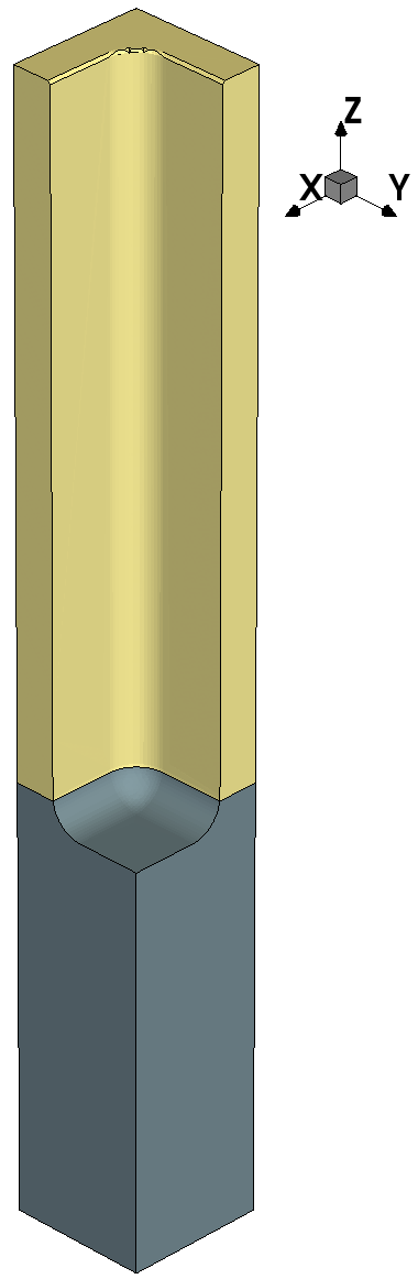
Figure 2. Etching using the parameterized simple RFM model m2. (Click image for full-size view.)

The advantage of model m2 in comparison to model m1 is that the value of the etching rate now can be varied when configuring an etching machine. Therefore, model m2 can be reused easily in different applications; whereas, model m1 would need to be modified for each new application.

4.1.3 Modeling a Material-Dependent Etching Rate

In the model m2 introduced in Section 4.1.2 Modeling Isotropic Etching With Parameters, the etching rate was assumed to be the same for all materials. A more realistic model would take into account the dependency of the etching rate on the etched material. This can be achieved with the RFM by defining a parameter as follows:

add_float_parameter ... scope=material_dependent default=0 ...

When configuring a machine, since the scope of the parameter etch_rate is set to material_dependent, its value is not set with the define_etch_machine command, but with the add_material command, as follows:

define_etch_machine model=m3
add_material material=Photoresist etch_rate=@<etch_rate*0.001>@
add_material material=Silicon etch_rate=@<etch_rate>@

Here, the define_etch_machine and add_material commands configure a machine using the model m3.

The value of the parameter etch_rate is set to 0.001x@etch_rate@ μm/minute for photoresist and @etch_rate@ μm/minute for silicon; whereas, the default value (0 μm/minute) will be used for the other materials present in the structure, if any.

The default values of the parameters are provided in the model definition. However, when a machine is configured, the values of the parameters can be overwritten with any value in the allowed range.

The complete example is:

# Model definition.
define_model name=m3 type=etch \
  description="An etch model with material-dependent etch rate"
add_float_parameter name=etch_rate model=m3 \
  default=0 min=0 scope=material_dependent quantity=velocity
add_formula model=m3 expression="-etch_rate()"
finalize_model model=m3
# Machine configuration.
define_etch_machine model=m3
# Specify the value of "etch_rate" for photoresist and silicon.
# The default value of "etch_rate" is used for all other materials.
add_material material=Photoresist etch_rate=@<etch_rate*0.001>@
add_material material=Silicon etch_rate=@<etch_rate>@
define_structure material=Silicon point_min={0 0 0} point_max={0.1 0.1 0.3}
define_shape type=cube name=mask point_min={0.0 0.0 0.3} \
	point_max={0.1 0.1 0.8}
deposit shape=mask material=Photoresist
define_shape type=cube name=trench point_min={0.05 0.05 0.3} \
	point_max={0.1 0.1 0.8}
etch shape=trench
save file=n@node@_init.tdr
etch spacing=0.002 time=1.0
save

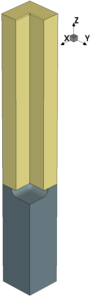
Figure 3. Etching using the simple RFM model m3 with a material-dependent rate. (Click image for full-size view.)

4.1.4 Using a Material-Dependent Rate Formula

Material-dependent parameters take into account differences in the properties of materials. The RFM provides a different mechanism to model material-dependent behaviors: material-dependent rate formulas. This means that different mathematical expressions can be used to compute the process rates on different materials.

To provide an example of this RFM capability, suppose that a model must be defined in which silicon will be etched only if visible from the vertical direction, at a rate proportional to the cosine of the angle between the normal of the surface element and the vertical direction. All other materials will be etched isotropically. Here is a complete example that defines such a model and runs a simulation based on it:

define_model name=m4 type=etch \
  description="An etch model with material-dependent rate formula"
add_float_parameter name=etch_rate model=m4 default=0 min=0 \
  scope=material_dependent quantity=velocity
# Specify the default mathematical expression of the rate.
add_formula model=m4 expression="-etch_rate()"
# Specify the mathematical expression of the rate to use for silicon.
add_formula model=m4 material=Silicon \
  expression="-etch_rate() * cos(theta()) * visible()"
finalize_model model=m4
define_etch_machine model=m4
add_material material=Photoresist etch_rate=@<etch_rate*0.001>@
add_material material=Silicon etch_rate=@<etch_rate>@
define_structure material=Silicon point_min={0 0 0} point_max={0.1 0.1 0.3}
define_shape type=cube name=mask point_min={0.0 0.0 0.3} \
	point_max={0.1 0.1 0.8}
deposit shape=mask material=Photoresist
define_shape type=cube name=trench point_min={0.05 0.05 0.3} \
	point_max={0.1 0.1 0.8}
etch shape=trench
save file=n@node@_init.tdr
etch spacing=0.002 time=1.0
save

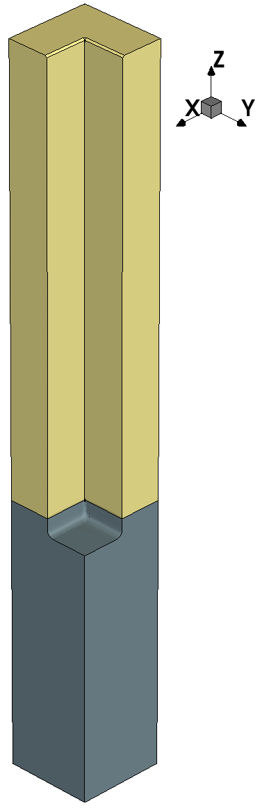
Figure 4. Etching using the simple RFM model m4 with a material-dependent formula. (Click image for full-size view.)

In this example, a default rate formula is defined along with a rate formula specific for silicon, specified with the material parameter in the add_formula command.

The following RFM built-in functions are used in such an expression:

cos() returns the cosine of an angle expressed in radian.
theta() returns the angle in radian between the vertical direction and the normal of the element to which the formula is applied.
visible() returns 1 if the surface element to which the formula is applied is visible from the vertical direction, and 0 otherwise.

The same model could have been described without using material-dependent rate formulas, but only material-dependent parameters. Nevertheless, the use of a material-dependent rate formula has advantages:

The number of parameters is reduced.
The model is easier to write and to understand.
The information that the visibility is relevant only for silicon is directly included in the model, and it is then clear that only one parameter must be calibrated for each material.

4.2 Flux Models

These examples of creating different simple RFM models involve different fluxes.

The complete project can be investigated from within Sentaurus Workbench in the directory Applications_Library/GettingStarted/sptopo3d/RFM_Flux_Models.

4.2.1 Modeling Neutral Fluxes

The RFM allows you to include fluxes of particles and the related physical effects into a user-defined model.

In the following example, this feature is demonstrated by setting up a model for the configuration of Figure 5, which describes a process to deposit silicon oxide at a rate proportional to the total flux of some neutral particles.

To include a neutral flux in an RFM model, the add_neutral_flux command is used in the definition of the model.

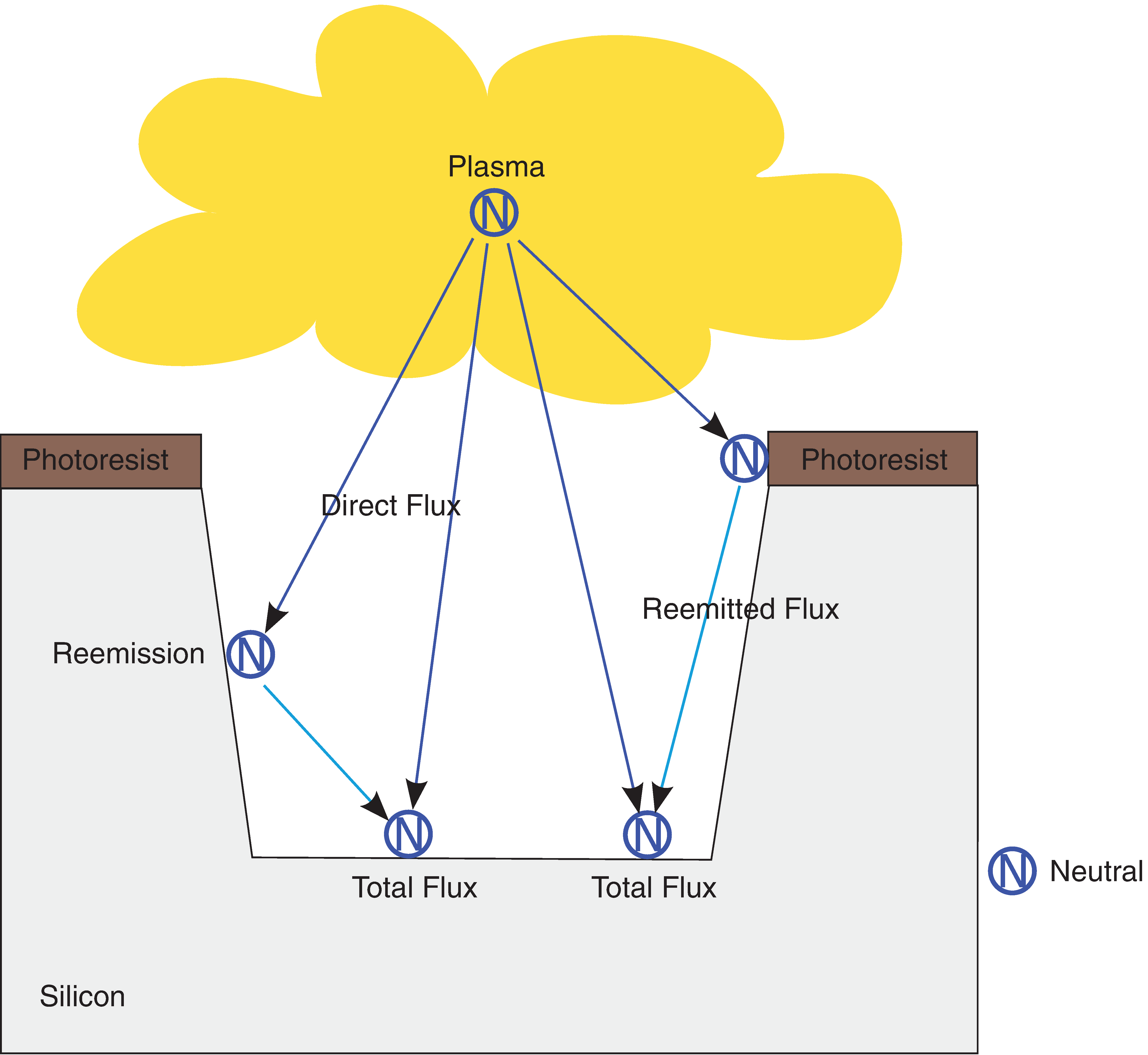
Figure 5. Deposition process involving a neutral flux; reemission of neutrals from surface is taken into account. (Click image for full-size view.)

If the model is called m5 and the flux of neutrals is called N, the model can be defined with the commands:

define_model name=m5 type=deposit \
  description="A deposition model with deposition rate \
  proportional to the total flux of neutrals"
# Define a flux of neutrals called "N".
add_neutral_flux name=N model=m5
add_float_parameter name=deposition_rate model=m5 min=0 scope=global \
  quantity=velocity
# Use the total flux of "N" in the rate formula definition.
add_formula model=m5 expression="deposition_rate() * total_flux(N)"
finalize_model model=m5

The value of the total flux is obtained in the rate formula using the total_flux() RFM built-in function and passing the name of the flux to it as an argument. Moreover, since this is a deposition model, the sign of the rate is positive.

When a deposition machine is configured with such a model, the value of the sticking coefficient for the flux N is provided using the add_flux_properties command.

Since m5 is a deposition model, the sticking coefficient cannot be material dependent. Analogously, material-dependent parameters are not allowed in deposition models either.

The commands to define a deposition machine using the model m5, to set the sticking coefficient for flux N, to define the initial structure, and to run the simulation are:

define_deposit_machine model=m5 material=Oxide deposition_rate=@depo_rate@
add_flux_properties flux=N sticking=0.7
define_structure material=Silicon point_min={0 0 0} point_max={0.1 0.1 0.3}
define_shape type=cube name=trench point_min={0.05 0.05 0.1} \
	point_max={0.1 0.1 0.3}
etch shape=trench
save file=n@node@_init.tdr
deposit spacing=0.005 time=1.0 engine=monte_carlo
save

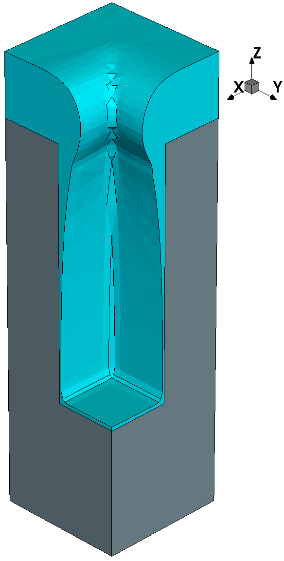
Figure 6. Etching using a neutral flux in the deposition RFM model m5. (Click image for full-size view.)

4.2.2 Modeling a Neutral Flux and an Ion Flux

In this section, an etching model using a neutral flux and an ion flux is set up.

Figure 7 shows the considered configuration, and the etching rate is assumed to be proportional to the product between the total flux of neutrals and the direct flux of ions. In this way, an interaction between the two different species is taken into account.

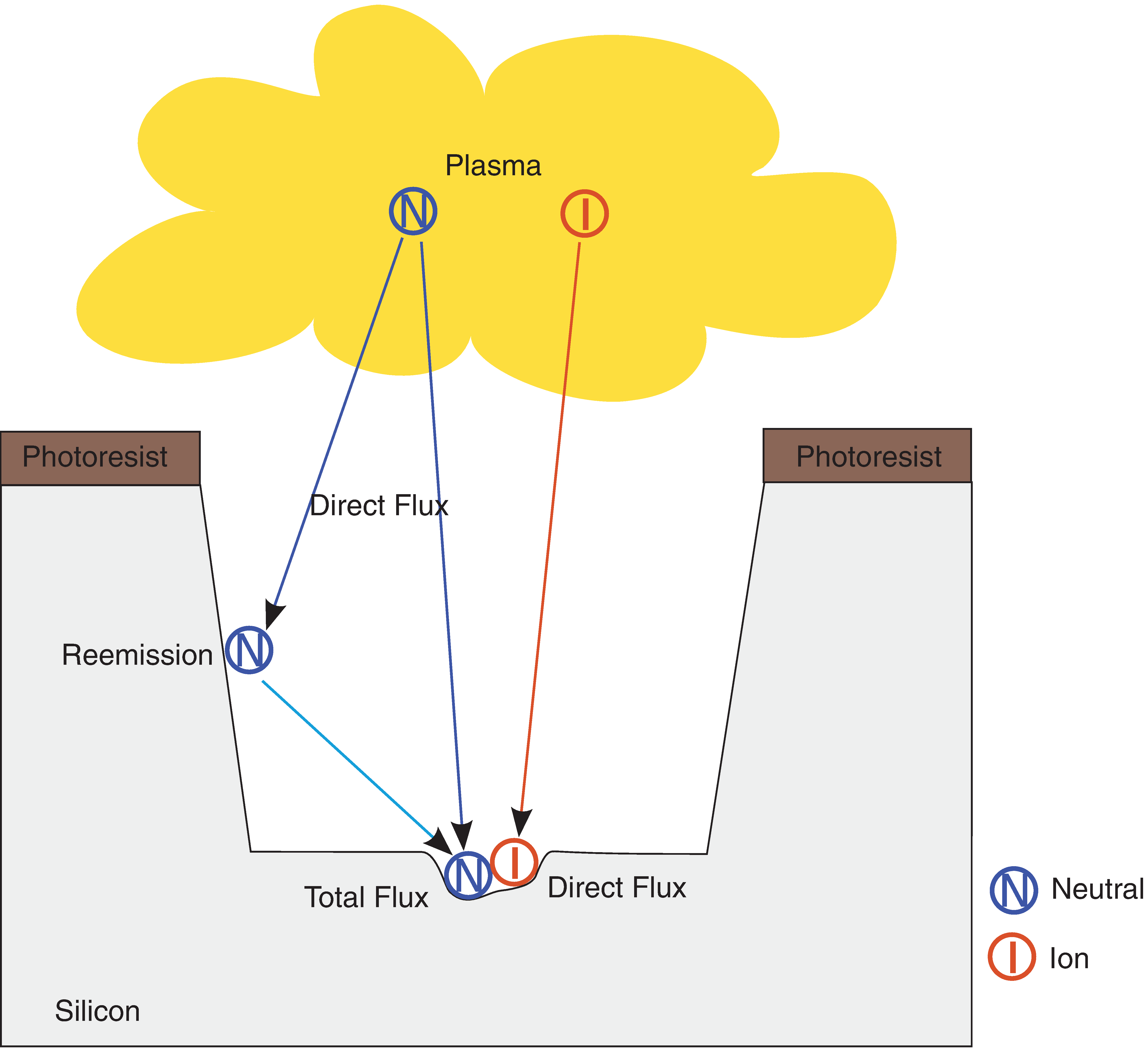
Figure 7. Etching process involving a neutral flux and an ion flux that interact with each other; reemission from the surface is taken into account for neutrals; reflection, sputtering, and sputter deposition are not taken into account for the ion flux. (Click image for full-size view.)

For simplification, interactions of ions with the surface are not taken into account in this model. Therefore, reflection, sputtering, and sputter deposition are deactivated in the add_ion_flux command. Accordingly, the model m6 can be defined as follows:

define_model name=m6 type=etch \
  description="An etch model involving neutrals and ions"
add_neutral_flux name=N model=m6
# Define an energy-independent ion flux called "I"
# with no physical effect enabled.
add_ion_flux name=I model=m6 energy=independent reflection=false \
  sputtering=false
add_float_parameter name=etch_rate model=m6 default=0 min=0 \
  scope=material_dependent quantity=velocity
# Use the total flux of "N" and the direct flux of "I"
# in the rate formula definition.
add_formula model=m6 \
  expression="-etch_rate() * total_flux(N) * direct_flux(I)"
finalize_model model=m6

In the rate formula, the direct flux of the ion flux is obtained using the built-in RFM function direct_flux().

While the angular distribution of all neutrals is always assumed to be uniform, the angular distribution of any ion flux must be specified using the define_iad command.

In this example, the built-in cos^mθ distribution is used with an exponent of m=5000, as defined by the command:

define_iad name=my_iad species=I exponent=5000

To define an etching machine using the angular distribution my_iad, use:

define_etch_machine model=m6 iad=my_iad

To complete the example, the value of the sticking coefficient for the neutral flux N must be set as well as the value of the material-dependent parameter etch_rate.

Since m6 is an etching model, the sticking coefficient can be material dependent, as shown in the following example, which sets the sticking coefficient equal to 0.5 for silicon and 0.3 for photoresist:

# Set the value of the sticking coefficient for flux N.
add_flux_properties flux=N sticking=0.5 material=Silicon
add_flux_properties flux=N sticking=0.3 material=Photoresist
add_material material=Photoresist etch_rate=@<etch_rate/1000>@
add_material material=Silicon etch_rate=@etch_rate@
define_structure material=Silicon point_min={0 0 0} point_max={0.1 0.1 0.3}
define_shape type=cube name=mask point_min={0.0 0.0 0.3} \
	point_max={0.1 0.1 0.5}
deposit shape=mask material=Photoresist
define_shape type=cube name=trench point_min={0.05 0.05 0.3} \
	point_max={0.1 0.1 0.5}
etch shape=trench
save file=n@node@_init.tdr
etch spacing= {0.01 0.01 0.01} time=3.0 engine=monte_carlo 
save

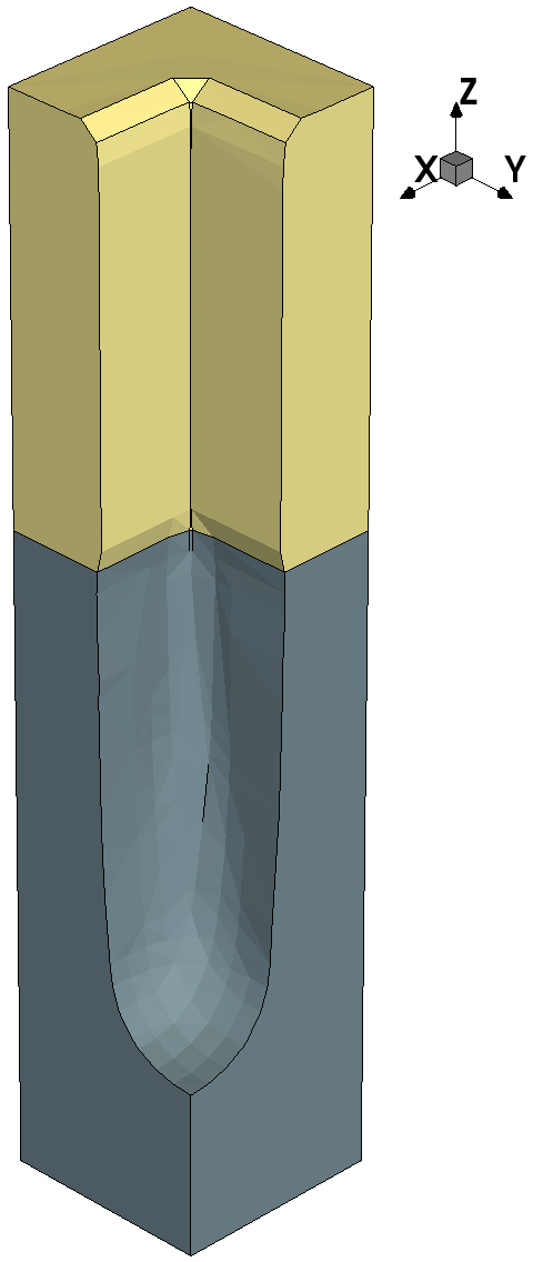
Figure 8. Etching using a neutral flux in combination with an ion flux in the etching RFM model m6. (Click image for full-size view.)

4.2.3 Modeling a Neutral Flux and an Ion Flux With Sputtering

Several physical effects are available for ions, but these effects were not activated in the previous example.

This example shows how sputtering by ions can be modeled with the RFM. The way of specifying the other available physical effects is similar.

Figure 9 shows the situation to be considered. It shows a simultaneous etching and deposition process in which etching occurs because of sputtering by ions, and deposition of silicon oxide occurs simultaneously due to neutral particles.

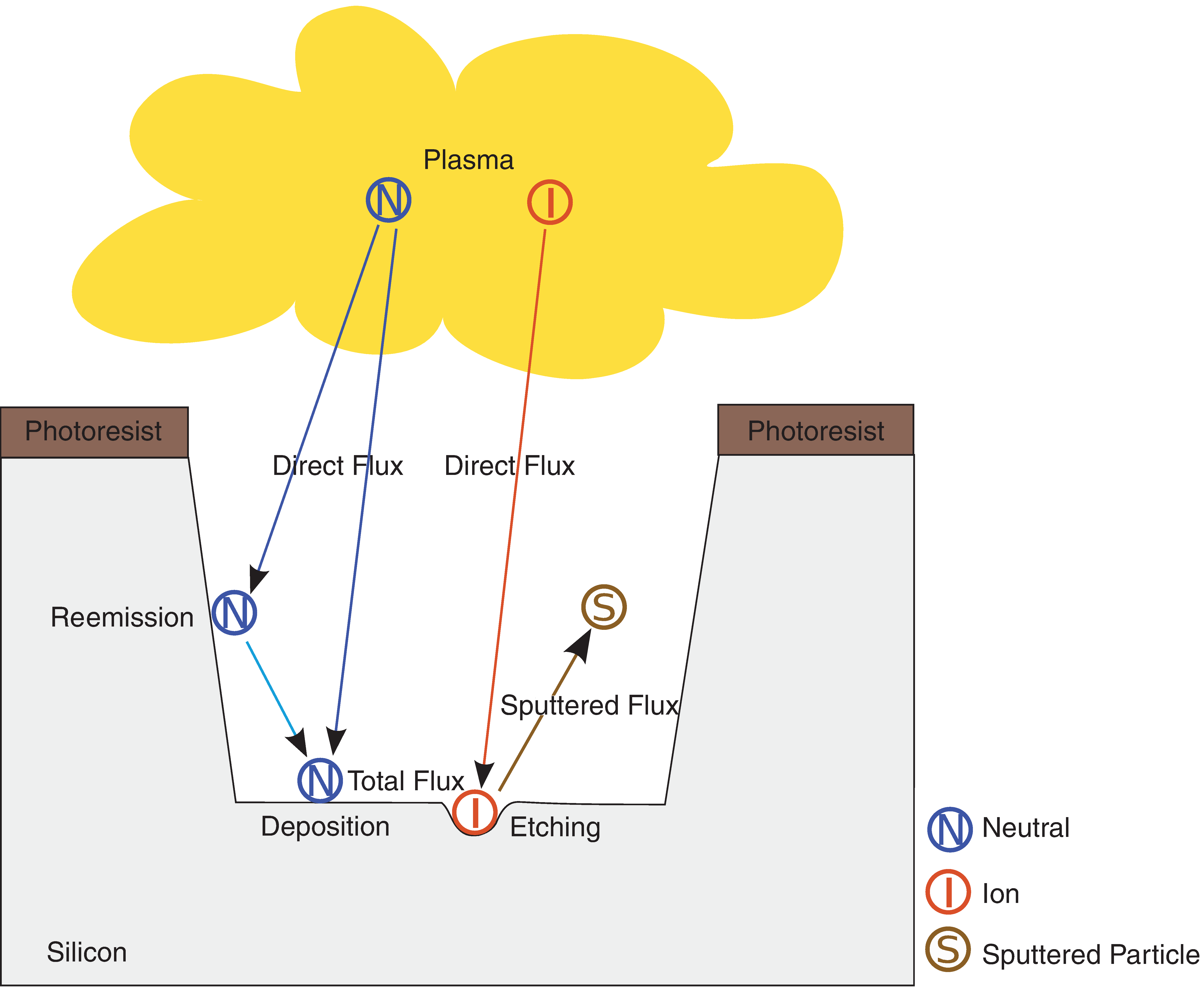
Figure 9. Simultaneous etching and deposition process involving a neutral flux and an ion flux; reemission of neutrals from the surface and sputtering by ions is taken into account; deposition is due to neutrals; and etching is due to ions. (Click image for full-size view.)

The etching rate is assumed to be proportional to the amount of material sputtered by ions; whereas, the deposition rate is supposed to be proportional to the total flux of neutrals.

To include sputtering in the model, first, such an effect must be activated by setting sputtering=true in the add_ion_flux command.

Moreover, a yield function must be specified to compute the amount of matter sputtered from each material present in the structure using the define_yield command.

Since yield functions depend also on the material with which the ions interact, the command define_yield has the parameter material to specify the target material.

A yield function according to Yamamura [Ref. 1] is assumed for silicon having a maximum yield of 2 when the angle between the incidence direction of ions and the normal of the surface element is equal to 35°. However, the yield function for photoresist is modeled using the Sentaurus Topography 3D model described by the parameters s1 and s2. Finally, since oxide is deposited, a yield function must be defined for oxide as well. A Yamamura model is used for this. The commands to define these functions are:

define_yield name=y species=I material=Silicon energy=0 theta_max=35 \
  yield_max=2
define_yield name=y species=I material=Photoresist energy=0 s1=5.5 s2=-6.0
define_yield name=y species=I material=Oxide energy=0 theta_max=60 \
  yield_max=1.4

The angular distributions, the yield functions, and the material to deposit are specified when an etching machine is defined with the command:

define_etch_machine model=m7 iad=my_iad yield=y \
        deposition_rate=@<etch_rate/100>@ deposit_material=Oxide

Click to view the complete command file rfm_neutral_ion_fluxes_sputtering_t3d.cmd.

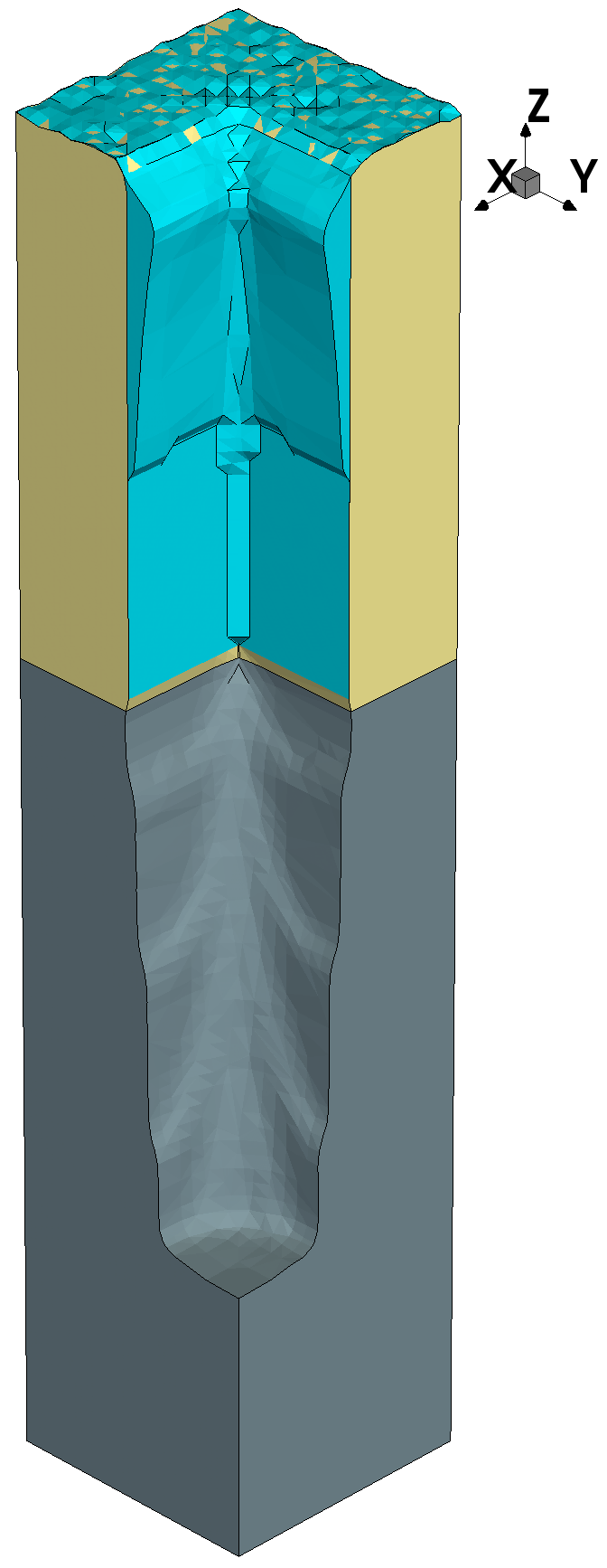
Figure 10. Neutral and ion fluxes used in RFM model m7 combined with sputtering. (Click image for full-size view.)

4.3 References

Ref. 1: T. K. Chini et al., "The angular dependence of sputtering yields of Ge and Ag," Nuclear Instruments and Methods in Physics Research Section B: Beam Interactions with Materials and Atoms, vol. 72, no. 3–4, pp. 355–358, 1992.