
Sentaurus Process
13. Special Focus: Lattice Kinetic Monte Carlo
13.1 General Considerations
13.2 LKMC Settings for the Simulation
13.3 Choosing an LKMC Model
13.4 Solid Phase Epitaxial Regrowth
13.5 Epitaxial Deposition
13.6 Understanding Information in the Log File
13.7 Using Advanced Calibration
13.8 References
Objectives
- To demonstrate how to use the lattice kinetic Monte Carlo method.
13.1 General Considerations
The lattice kinetic Monte Carlo (LKMC) method simulates on the atomistic scale the epitaxy of silicon and germanium, and simulates the solid phase epitaxial regrowth (SPER) of amorphous silicon to silicon. In this section, the term surface is used for the growing surface during epitaxy as well as the interface that separates crystalline and amorphous silicon in SPER. All such surfaces are represented by possible atom positions at and near that surface, with these positions being occupied or empty. The possible atom positions are arranged in a zinc-blende lattice (therefore, the term lattice KMC) and contain perfect lattice sites as well as possible defect sites (as in the case of twin defects).
The models of the LKMC method describe the interactions of atoms and molecules on such surfaces. For epitaxial growth, for example, the models describe how silane molecules interact with surface silicon atoms and then disintegrate, leaving new silicon atoms adsorbed to the surface. For SPER, the models describe how silicon atoms in an amorphous phase change their positions such that the crystalline region grows. In both cases, dopant diffusion can be modeled as well using the KMC diffusion method.
While in the LKMC method, all atoms at and near the surface are considered, the KMC diffusion method considers only defects and dopants (only atoms that do not belong to a perfect silicon or SiGe lattice).
Because the crystal structure and atom positions must be represented, all KMC and LKMC simulations are performed in three dimensions.
The LKMC method and the KMC diffusion method share some parameters, which are set with the command:
pdbSet KMC <parameter> <value>
Some of these settings are explained in this module. For more details, see Section 12. Special Focus: Kinetic Monte Carlo.
The examples chosen in this module are relatively simple to run within a reasonable time, yet they still illustrate the method.
For epitaxy, the growth of silicon from a silane-containing ambient, including doping, is used. Another epitaxy example grows a doped elevated source/drain region of a FinFET. For SPER, an example of recrystallization after ion implantation is demonstrated. A second example shows how an amorphous region with a fin-like structure is recrystallized.
13.2 LKMC Settings for the Simulation
For epitaxial deposition, the LKMC method can be used in full atomistic mode or in hybrid mode. Full atomistic means dopants are modeled using the KMC method, while the growing surface is modeled using the LKMC method. To use the full atomistic mode, specify:
SetAtomistic
pdbSet LKMC Epitaxy true
To use the hybrid mode, specify the option lkmc in the diffuse command. With that, the epitaxial growth is modeled atomistically during this diffusion step, and dopant diffusion is modeled in continuum mode. The hybrid mode can be used if you are interested only in the shape of the grown region.
SPER is modeled using the KMC method if SetAtomistic is specified. The KMC method uses a simple isotropic model. To use the LKMC method, you must specify one of the LKMC models as follows:
pdbSet Silicon KMC damage SPER.model <model>
where <model> is one of the SPER models listed in Section 13.3 Choosing an LKMC Model (see Table 1).
| Model | Method | Switch on using | Dopant diffusion | Use for |
|---|---|---|---|---|
| Epitaxy | Hybrid | diffuse ... lkmc | Continuum | Si or SiGe elevated source/drain shape |
| Epitaxy | Full atomistic | SetAtomistic pdbSet KMC Epitaxy true |
Using KMC | Si or SiGe elevated source/drain with accurate doping |
| SPER | Simple KMC | SetAtomistic | Using KMC | Full atomistic flow with simple SPER model |
| SPER | KMC and LKMC | SetAtomistic pdbSet Silicon KMC Damage SPER.model <model> |
Using KMC | Full atomistic flow |
As noted in Section 13.1 General Considerations, LKMC simulations are always performed in three dimensions. You must specify the depth of the simulation domain, that is, the thickness of the substrate to be simulated. For the lateral directions, the following default settings can be overwritten:
pdbSet KMC MaxYum 0.04
pdbSet KMC MaxZum 0.04
MaxYum is the size of the KMC or LKMC simulation domain (in μm) in the y-direction. Similarly, MaxZum is the size of the simulation domain in the z-direction.
13.3 Choosing an LKMC Model
The models implemented for LKMC SPER are:
- The Planes model is a basic LKMC model parameterized using the crystal orientation.
- The Coordinations.Planes model can be extended to account for the local atomic configuration. Currently, it is parameterized using only crystal planes.
The model for SPER is selected by specifying:
pdbSet <material> KMC Damage SPER.Model <model>
The Planes model is used, in this section, for SPER.
The models implemented for epitaxial deposition are:
- The Coordinations.Reactions model and the Coordinations model are based on atomic bonding energies.
- The Planes model and the Coordination.Planes model are based on the local surface orientation.
The growth rates and the reaction rates in the Coordinations.Reactions and Coordinations models are determined by the coordination, that is, the number and the type of bonds between the depositing species and those on the surface. In addition, the Coordinations.Reactions model considers reactions that occur during chemical vapor deposition. Examples of such reactions include the decomposition of source gases, the site blocking effects of a carrier gas such as H2, and the desorption of source gas molecules. The Coordinations model does not consider reactions, but it includes the growth rate dependency on the composition and the crystal orientation of the deposition surface.
The model for epitaxial deposition is selected by specifying;
pdbSet LKMC Epitaxy.Model <model>
where <model> can be one of the following:
- Coordinations
- Coordinations.Planes
- Coordinations.Reactions
- Planes
The Coordinations.Reactions model is used, in this section, for epitaxial deposition.
13.4 Solid Phase Epitaxial Regrowth
The easiest way to start with SPER in the LKMC method is to use an existing KMC simulation setup. With that, you can use all the KMC framework (data extraction and so on) of the KMC simulation. The only additional line needed is:
pdbSet Silicon KMC Damage SPER.Model Planes
which couples the LKMC recrystallization to the KMC simulation. Such a derived example is located in Applications_Library/GettingStarted/sprocess/LKMC_SPER_snowplough.
The present example is based on the KMC simulation in Section 12. Special Focus: Kinetic Monte Carlo. Here, an amorphizing germanium implantation step is followed by indium implantation. The subsequent diffusion step is performed with the LKMC method switched on. At the end of the simulation, two TDR files are written:
kmc extract tdrWrite filename=n@node@_anneal
...
struct tdr=n@node@
The first file is written using the KMC method and contains all the information discussed in Section 12. Special Focus: Kinetic Monte Carlo.
The second file contains all the atomistic information at the end of the simulation (see Figure 1). The top part of the silicon is still amorphous (indicated in light red). It is separated from the crystallized region (light blue) by the crystallization front (silicon atoms shown in green). All individual silicon atoms at the crystallization front are modeled explicitly. Recrystallization starts also from the surface. The green islands on the top are silicon atoms at the amorphous/crystalline interface. Immediately below the amorphous interface, there are few defects. The amorphous silicon has recrystallized to an almost perfect silicon lattice containing some indium atoms (purple spheres) and a few point defects (red spheres).
Further down, a region with a high number of interstitials, vacancies, and extended defects (red and green spheres) starts at the location up to which the silicon was amorphized due to the germanium implantation.
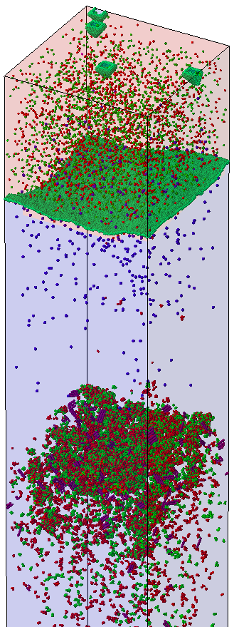
Figure 1. SPER after indium ion implantation. (Click image for full-size view.)
For the second SPER example (Applications_Library/GettingStarted/sprocess/LKMC_SPER-2Dfin), a simple 2D structure is used that represents a cross section of a fin in FinFET technology. A high concentration of Frenkel pairs is defined to make the silicon amorphous in the fin. The Coordinations.Planes model is switched on to model SPER. With that, the diffusion step is performed with the LKMC method. Figure 2 shows several snapshots taken during the diffusion. Because of the orientation dependency of the growth rates (the 111 direction has the slowest rate), you can observe the characteristic facet formation.
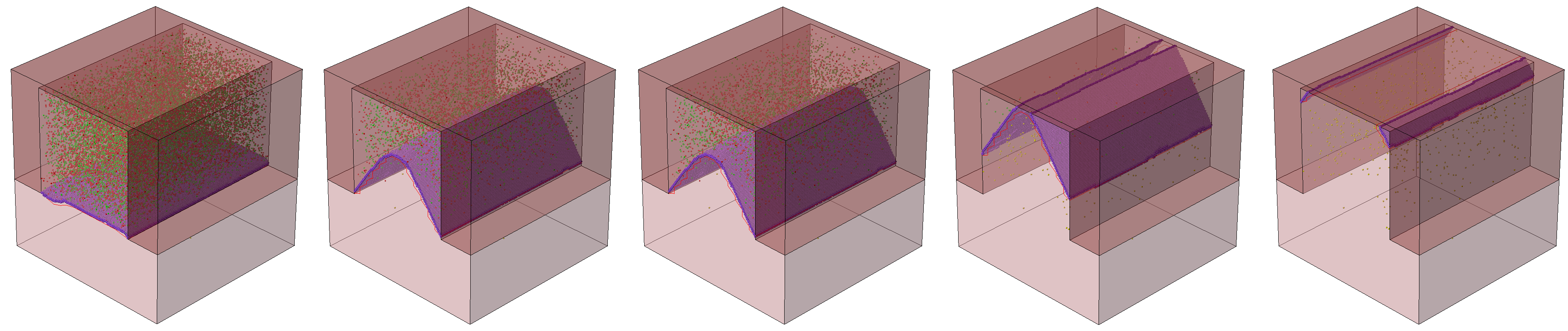
Figure 2. Snapshots taken during SPER after (left to right) 5 s, 15 s, 50 s 100 s, and 200 s: interstitials (red), vacancies (green), and silicon atoms (purple) at the recrystallization front, and twin defects (yellow). (Click image for full-size view.)
The regrown crystalline silicon is not completely defect free. During the crystallization, several defects can form. In the LKMC method, you take into account the formation of twin defects on the 111 plane as described in [Ref. 1]. As mentioned in Section 13.1 General Considerations, the simulator represents the volume around a growing surface by lattice sites being occupied during growth. Here, lattice sites are perfect lattice sites and twin-defect sites. The local atomistic configuration of a twin defect is shown in Figure 3. The probability to form such a twin defect is set using:
pdbSet KMC Si Damage probability.SPER.defect <n>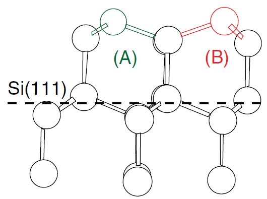
Figure 3. Perfect silicon lattice is highlighted in green (A) and twin defect is highlighted in red (B). (Click image for full-size view.)
In the LKMC or KMC method, twin defects do not interact with other defects. They are mainly an indication where and under which conditions defective silicon forms. You can find the number of twin defects using the kmc extract command, for example:
set NDefect [kmc extract defects name=I
defectname=TwinDefect countparticles]
puts "DOE: twins $NDefect"
Here, the second command puts the extracted number into the Sentaurus Workbench table.
13.5 Epitaxial Deposition
For epitaxial deposition, you first use a simple 1D example, Applications_Library/GettingStarted/sprocess/LKMC_Depo_SiP. The gas flows and the annealing steps are defined by the following commands:
gas_flow name= SiP epi flowHGas=1000 flowDichlorosilane=50 \
         flowPhosphine=30 pressure= 20<torr>
temp_ramp name= SiPEpi gas.flow= SiP epi.model=1 \
          time= 1.0 temp=700
diffuse temp.ramp=SiPEpi info=0
With this, an epitaxial deposition step for 1 minute at 700°C is simulated. Hydrogen is used as the carrier gas, and the gas contains SiH2Cl2 to grow silicon and PH3 for the silicon doping. The units for the gas flows follow the Sentaurus Process convention. There are more predefined gases available, and you can define a new gas as well.
You want to model the reactions explicitly on the surface, so you use the Coordinations.Reactions model. At any given time during the simulation, several atomic and molecular species can be found on the surface, as shown in Figure 4.
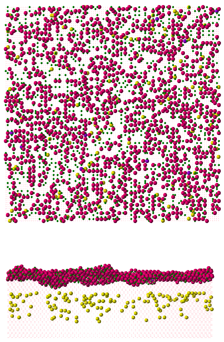
Figure 4. (Top) A top view during the simulation showing Si surface atoms (green), HStar on the surface (red), SiCl2Star (purple), and phosphorus (yellow); (bottom) view along the 110 direction with silicon lattice atoms shown as dots. (Click image for full-size view.)
The second example Applications_Library/GettingStarted/sprocess/LKMC_25nmFinFET for epitaxial growth is a 3D FinFET in which the deposition of the highly doped source and drain areas is modeled using the LKMC method. The epitaxial step is embedded into a continuum diffusion process flow.
To start the epitaxial growth in the LKMC method, you switch on the atomistic mode and chose the model as follows:
SetAtomistic
pdbSet LKMC Epitaxy.Model Coordinations.Planes
With this, the growth is modeled using the LKMC method. Existing dopant concentrations are converted to individual atoms. These and the dopants introduced during the growth are modeled using the KMC method. Figure 5 shows the time evolution of this simulation.
The simulation is performed in full atomistic mode. It is recommended to stay in this mode until the end of the simulation.
After the LKMC growth, the atomistic structure of the grown surface must be converted into a continuous boundary. The accuracy of this conversion is controlled by the following parameter:
pdbSet KMC Simplify.Geometry 1.0E-4
Higher values will lead to smoother surfaces, and lower values lead to better resolution. Better resolution typically leads to more mesh nodes.
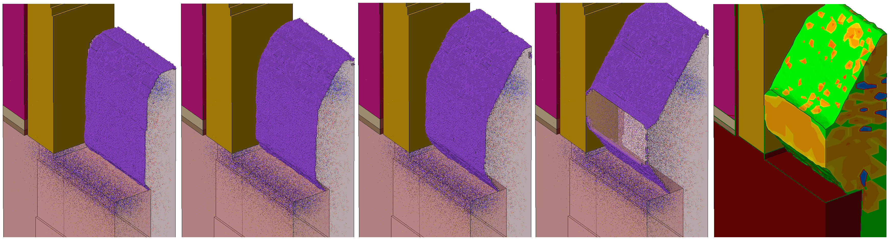
Figure 5. Time evolution of the LKMC deposition: the structure is shown after (left to right) 1 minute, 2 minutes, 3 minutes, 4 minutes, and 5 minutes; purple spheres represent the surface, colored dots are dopant ions, and (far right) structure shows the conversion to continuum dopants and boundary. (Click image for full-size view.)
13.6 Understanding Information in the Log File
The log file contains information about the models used:
SPER model | Lattice KMC
For the epitaxial growth, it reads:
pdbSet LKMC Epitaxy.Model Coordinations.Reactions
Since you are using the Coordination.Reactions model, the list of possible reactions is printed, for example:
Name: PH2Star_sr
              type: SurfaceReaction
         prefactor: 100(1/s)
            energy: 0(eV)
    max separation: 0.41(nm)
          ambients: *0
         reactants: 1*PH2Star
          products: 1*Phosphorus
       segregating:
The name of the reaction is PH2Star_sr, where the sr suffix indicates it is a surface reaction. Other possible suffixes for built-in reactions are ads (adsorption), des (desorption), and etch (etching). All reactions describe the reaction of a reactant (here, PH2Star) with the surface. The product here is one phosphorus atom (on the surface) and two hydrogen atoms released to the ambient gas. Atoms released to the gas are removed from the simulation.
At the end of the diffusion step, the KMC and LKMC reports are written to the log file. The KMC reports are explained in Section 12. Special Focus: Kinetic Monte Carlo.
The LKMC method writes an activity report and an event report. The activity report looks like:
--            LKMC activity report                        --
First:  Time Events   Temp |  Last: Time     Events Temp  Cleaned    Label
       0.000 0.00e+00  700 |   110555 here                     0     Silicon
5.322274e-03 2.66e+03  700 |      997 here                     0  Phosphorus
1.030382e-06 1.00e+00  700 |     1291 here                  7958       HStar
1.904441e-04 1.81e+02  700 |        59.956 7.74e+05  700       7     PH2Star
2.061115e-06 2.00e+00  700 |        9 here                   489   SiCl2Star
The first column prints the time at which a particular LKMC atom is observed. Here, you have silicon at the initialization of the LKMC method (time=0). The first phosphorus atom was observed at 5.32e-3 s.
At the end of the diffusion, there are 110555 silicon atoms and 997 phosphorus atoms, and the HStar, PH2Star, and SiCl2Star reactants are listed. The Cleaned column lists the species that are discarded from the simulation, for example, 7958 HStar ions were discarded when they were found to be buried inside the silicon.
The LKMC event report looks like:
-- LKMC event report --
Name: Phosphine_ads        #Events:     1004
      Type: Adsorption
      Ambients:  Phosphine 1
      Products:  1 PH2Star
This report lists the number of events performed for each species during the simulation. Here, 1004 events of phosphine adsorption on the surface were simulated, involving phosphine from the ambient and resulting in a PH2Star being adsorbed on the silicon surface.
13.7 Using Advanced Calibration
The best generally available parameter set for the KMC method and the LKMC method is contained in the file AdvCal_KMC_2022.12.fps.
For a simulation flow that starts with continuum diffusion and later switches to use the KMC or LKMC method, it is recommended to set the following:
AdvancedCalibration    ;# loads the Advanced Calibration file for continuum
SetAtomistic
AdvancedCalibration    ;# loads the Advanced Calibration file for KMC/LKMC
UnsetAtomistic
<continuum process flow>
SetAtomistic
<KMC or LKMC flow>
13.8 References
- Ref. 1
- I. Martin-Bragado and B. Sklenard, "Understanding Si(111) solid phase epitaxial regrowth using Monte Carlo modeling: Bi-modal growth, defect formation, and interface topology," Journal of Applied Physics, vol. 112, no. 2, p. 024327, 2012.
Copyright © 2022 Synopsys, Inc. All rights reserved.