
Sentaurus Process
12. Special Focus: Kinetic Monte Carlo
12.1 General Considerations
12.2 Simulation Example
12.3 KMC Settings for the Simulation
12.4 Starting the Simulation
12.5 Comparing Simulation Results to Measurements
12.6 Extracting Further Information
12.7 Visualizing Results
12.8 Understanding Information in the Log File
12.9 Improving Resolution of Concentrations
12.10 References
Objectives
- To demonstrate the kinetic Monte Carlo (KMC) module of Sentaurus Process.
12.1 General Considerations
Sentaurus Process Kinetic Monte Carlo (Sentaurus Process KMC) models individual impurity atoms and individual point defects. Extended defects are modeled as aggregates of individual impurity defects and point defects in all combinations. This is in strong contrast to continuum modeling, which considers concentrations.
Since Sentaurus Process KMC deals with individual atoms and defects, it does not need a mesh, unlike continuum simulators. Nevertheless, it sets up a different kind of mesh, which is needed to define a list of particles that can interact with each other.
You can think of the KMC mesh as the simulation domain divided into a number of boxes. These boxes are created automatically. There is usually no need for users to influence the size or the number of these boxes. Another important difference to continuum simulations is that KMC simulations are always performed in three dimensions. This is a direct consequence of the fact that the simulation deals with individual particles. So, even if you want to simulate a quasi-one-dimensional (1D) structure (for comparison to SIMS measurements, for example), the simulation is performed internally in three dimensions.
Because of all these differences, switching between atomistic simulation and continuum simulation requires special attention.
12.2 Simulation Example
Here, a simple example demonstrates the most important issues that users must deal with when using Sentaurus Process KMC.
A commonly occurring situation is a quasi-1D simulation of an implantation followed by an annealing step to compare simulation results with measurements. Here, a simulation for an amorphizing implantation of germanium is performed, followed by a low-energy boron implantation and a long-time, low-temperature anneal. Experimental results have been published by Duffy et al. [Ref. 1]; a comparison of the KMC simulation results to these experiments was performed by Zographos et al. [Ref. 2]. In both papers, a certain range of implantation and annealing conditions was considered.
In this example, however, the use of Sentaurus Process KMC is illustrated only for one particular condition. This particular example was chosen for several reasons:
- The simulation time is sufficiently short.
- The experimental conditions show a wide range of phenomena that are within the scope of a KMC simulation (amorphization, recrystallization, uphill diffusion, and extended defects).
- Experimental results are available for comparison.
The example is simple but demonstrates everything needed in more complex cases.
The complete project can be investigated from within Sentaurus Workbench in the directory Applications_Library/GettingStarted/sprocess/KMC.
12.3 KMC Settings for the Simulation
The structure is set up as for a continuum simulation. Several switches control Sentaurus Process KMC and the output of the simulation. All of these switches have defaults, so it is unnecessary to set all of them explicitly. In this example, some of the most commonly switches are set and explained.
The parameters for the KMC simulation can be divided into three groups:
- Those for setting the size of the simulation domain.
- Those for setting the simulation temperature.
- Those for controlling the output.
12.3.1 Parameters for Setting the Size of the Simulation Domain
As mentioned in Section 12.1 General Considerations, the simulation is always performed in three dimensions. Sentaurus Process expects users to specify the depth of the simulation domain (that is the thickness into the silicon that must be simulated). For the lateral directions, there are default settings that can be overwritten:
pdbSet KMC MaxYum 0.04
pdbSet KMC MaxZum 0.04
MaxYum is the size of the KMC simulation domain (in μm) in the y-direction, and similarly MaxZum is the size of the domain in the z-direction. The size of the simulation domain must not be too small. The depth should be such that the simulation results are independent of it. For a typical application, this is the case for a depth of 0.75 μm or more, which is deeper than the depths to which fast point-defects diffuse.
The depth of the simulation domain has a small impact on the simulation time because time is spent only to simulate particles. If there are only a few particles at the bottom of the structure, they have a negligibly small effect on the simulation time.
The lateral dimensions of the simulation cell must be wide enough so that both implantation cascades and extended defects can form freely. This condition is satisfied if the size of a cascade or an extended defect is smaller than half the size of the simulation domain. As you will see in Section 12.4.1 Ion Implantation, the lateral size of the simulation domain strongly influences the simulation time. In Section 12.9 Improving Resolution of Concentrations, you will see that the lateral size also influences the noise level of the simulation. Here, the lateral dimensions are chosen to be 40 nm, which is sufficiently large for all defects and cascades to form, and small enough to allow a short simulation time.
12.3.2 Parameters for Setting the Simulation Temperature
In a continuum simulation, effects at or around room temperature are usually not modeled. In a KMC simulation, phenomena at room temperature must be considered such as dynamic annealing during implantation. Therefore, the temperature at which the implantation is performed must be set, and the temperature ramp rate until the subsequent annealing temperature is reached can be set as follows:
pdbSet KMC automaticRampUp   1
pdbSet KMC rampUpRate        100
pdbSet KMC automaticRampDown 1
pdbSet KMC rampDownRate      50

pdbSet MCImplant Temperature 300.0
Here, the temperature at which the ion implantation is performed is specified to be 300 K. Then, automatic ramp-up and ramp-down is switched on by Boolean arguments: the ramp-up with a rate of 100 K/s, and the ramp-down with a rate of 50 K/s. With these settings, the temperature can change continuously during the simulation, and you can specify annealing cycles in the same way as continuum simulations (and starting, for example, at 700°C).
12.3.3 Parameters for Controlling the Output
You can collect information during KMC simulations and can save all the collected information when the simulation is finished. The most frequently changed parameters are:
pdbSet KMC maxSnapshots 3
pdbSet KMC Decade 3
pdbSet KMC Movie { kmc extract tdrAdd defects concentrations histogram}
A snapshot is a set of particle positions at a given time. With the above settings, only one snapshot is kept in the computer memory. The next statement specifies that snapshots should be taken on a logarithmic time scale (Decade). In this example, three snapshots per time decade are kept in the memory (three from 1 s to 10 s, three from 10 s to 100 s, and so on, but only the last snapshot is kept).
The logarithmic time scale is usually taken because most changes occur in the first part of any annealing cycle. Alternatively, you can switch to a linear time scale (by replacing Decade with Every, and specifying the number of events after which a snapshot is written). These settings specify only at which times the snapshots of the simulation should be taken; the time step of the simulation is not influenced by these parameters.
The third statement specifies what should be saved in these snapshots. With defects, atomistic information will be saved (that is, particle positions). With concentrations, a conversion of atomistic data to continuum fields will be performed. With histogram, information about the distribution of certain cluster sizes will be saved. See Section 12.7 Visualizing Results for examples.
12.4 Starting the Simulation
To switch on the KMC model implemented in Sentaurus Process, use:
SetAtomistic
With this command, any existing field will be atomized, and implantation and diffusion are performed by Sentaurus Process KMC. The next command loads a file with calibrated parameters:
AdvancedCalibration
This file contains the recommended set of models and parameters calibrated to deep-submicron CMOS technology. The next lines (not shown here) define a mesh for a continuum simulation. This is needed for the structure representation and when the atomistic information is converted to field data. With the definition of the continuum mesh, you specify also whether the simulation will be performed internally in three dimensions (if the continuum mesh is specified only for one or two dimensions) or explicitly in three dimensions (if a 3D continuum mesh is specified). In this example, a 1D mesh is used because a simple comparison of 1D simulation results to 1D SIMS data is required. The process simulation steps are specified in the same way as for a continuum simulation.
12.4.1 Ion Implantation
With the SetAtomistic command, the following simulation steps will be performed in atomistic mode. This means that the ion implantation is performed using the Monte Carlo method. There are, however, several differences to the use of the Monte Carlo implantation method in a continuum diffusion simulation.
First, every ion implanted in the KMC mode represents a real ion. This means that the number of ions to be implanted is calculated from the dose (specified in the implant command) and the surface area (specified explicitly by a 3D structure definition or implicitly if the structure is specified to be 1D). The number of ions is ions = dose x area. Therefore, in the present example, 19200 Ge ions (dose = 1.2e15 cm2) and 16000 B ions (dose = 1.0e15 cm2) are implanted onto a surface = 40 nm x 40 nm.
This is in strong contrast to the use of the Monte Carlo implantation mode together with continuum diffusion. In that case, every implanted ion represents the full dose, and the accuracy of the simulation can be increased by increasing the number of implanted ions.
Second, in KMC mode, the implantation is performed with a realistic time dependency. During the time of implantation, all possible events can already occur. Most of these events have a relatively low probability (since ion implantation is usually performed at room temperature). The annihilation event of an interstitial recombining with a vacancy is likely, however, and occurs frequently during implantation. This process is the dynamic annealing.
Third, ion implantation in KMC mode must be performed in full cascade mode. This means that the full process of implanted ions kicking out silicon ions from the lattice, and then these ions kicking out the secondary ions from the lattice, and so on, is considered. The switch to full cascade mode is set automatically.
12.4.2 Diffusion
Diffusion is performed in KMC mode because SetAtomistic is set. Annealing ramps are specified as in the continuum simulation mode. Model parameters are taken from the file AdvancedCalibration because this file is sourced after the SetAtomistic command.
Remember that automatic ramps from and to room temperature are switched on. The simulator input does not require any additional settings for this, similar to a continuum simulation.
12.5 Comparing Simulation Results to Measurements
One of the first things users usually want to do is to compare simulation results to experimental data. For this example, the simulation results are compared to the experimental results reported in [Ref. 1]. The experimental results were saved in ASCII files containing two columns: the depth (in μm) and the concentration (in cm-3). The experimental files contain one header line.
The files that contain the corresponding simulated data are written during the simulation. One file contains the total (chemical) boron concentration after the implantation step, and a second file contains the total boron concentration at the end of the annealing step. These files are written in the same way as for a continuum simulation:
SetPlxList {BTotal BActive}
WritePlx n@node@_asimplanted_cont.plx
The first command selects a list of fields, and the second command writes these fields into the specified file. When Sentaurus Process KMC is used, it is important to understand that this sequence maps the atomistic information onto the continuum mesh. This means that an averaging over the lateral dimensions is performed (because 3D positions must be mapped onto a 1D plot), and the assignment of particle positions onto mesh nodes in the third dimension (into the substrate) must be made.
The present example contains a Sentaurus Visual script that loads and displays the data from the simulation together with the experimental results, as shown in Figure 1. To reproduce this figure, select the corresponding Sentaurus Visual nodes and click the Run Selected Visualizer Nodes Together toolbar button.
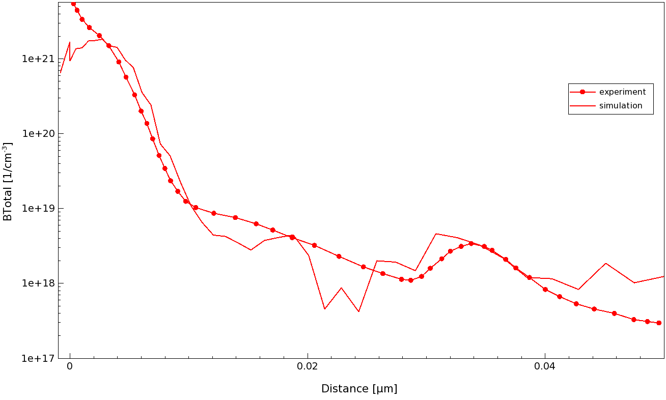
Figure 1. Experimental and simulated total boron profile after annealing. (Click image for full-size view.)
It is important to understand what the simulator does at this stage. For Sentaurus Process KMC, a simple "boron" particle does not exist. Instead, there are mobile boron particles in different charge states, substitutional boron, boron particles as part of dopant–interstitial clusters, and more.
Upon execution of the WritePlx command, Sentaurus Process KMC maps all these different types of boron particle onto a quantity that Sentaurus Process knows exists in a continuum diffusion model. With the command as above, all boron particles in all configurations are counted and mapped onto the field BTotal, which is in fact the total (chemical) boron concentration. With such a procedure, you can easily extract concentrations (fields) in the same way as for continuum simulations, and it is very easy to compare continuum results with KMC results. Similarly, active concentrations such as BActive, interface concentrations such as BInterface, and net active concentrations can be extracted.
There is one more important point that you must remember when extracting data. For any atomistic simulation, the result is a set of defects having individual coordinates. This result does not depend on the continuum mesh. However, the result of mapping these coordinates onto the continuum mesh does depend on this mesh. Figure 2 illustrates this effect. The KMC results are the same. They are mapped onto meshes with different spacing. The blue line uses a mesh with a spacing of 0.01 μm. This is too coarse and the peak of the concentration is not resolved at all. The red line uses a mesh spacing of 0.001 μm, and the green line uses a spacing of 0.0001 μm. The finer spacing does not bring any additional accuracy around the peak of the concentration. For lower concentrations, it only leads to more noise. This is because some of the small mesh elements might not contain any boron particles, which means that the concentration is zero. The next mesh element might contain only one boron particle but, since the mesh element is so small, the concentration is quite high.
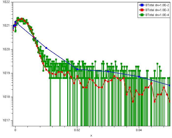
Figure 2. The effect of mapping atomistic data onto different meshes. Mesh spacings are 0.01 μm (blue), 0.001 μm (red), and 0.0001 μm (green). (Click image for full-size view.)
12.6 Extracting Further Information
The KMC method has the advantage that it delivers more information than a conventional simulation. All coordinates of all particles are known at any time step; therefore, you can extract profiles for any given defect at any time. In particular, you can extract profiles for all individual dopant–defect clusters, which are, in most continuum models, not taken into account individually. In the present example, you have:
set BTotal   [kmc extract profile name= Boron ]
set BCluster [kmc extract profile name= Boron defectname= ImpurityCluster]
set ll [list $BTotal "BTotal" $BCluster "BCluster"]
KMC2Plx $ll n@node@_asimpl_kmc.plx
The last command calls a Tcl procedure that is defined in the header of the command file; it writes data in the .plx format into a specified file. The second-last command is a Tcl command that puts certain data into a list. The first three lines use the Tcl command set to define variables (BTotal, BCluster, ThreeOneOne), and the value of these variables is defined to be the output of the command in brackets.
In the brackets, the kmc extract command extracts certain profiles. The first command extracts the profile Boron, which means all boron atoms in all possible configurations (charge state, whether it is part of a cluster, and so on) and, therefore, it extracts the total boron concentration.
The second command also extracts a boron profile, but it is restricted to boron atoms being part of an impurity cluster. The third command extracts all interstitials that are part of a {311} defect. The extraction of all these quantities is performed by mapping the atomistic information onto the KMC mesh in the vertical direction. In the lateral directions, the averaging is performed similarly to the method that uses WritePlx (as previously explained), but now the averaging is performed on the KMC mesh. Figure 3 shows the result of such an extraction.
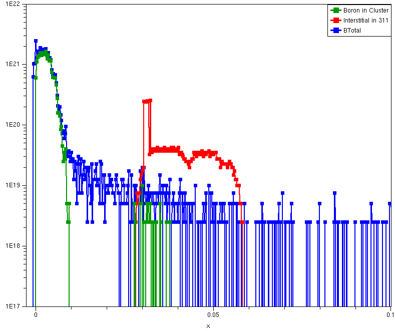
Figure 3. Total boron concentration (blue), interstitials belonging to {311} defects (red), and boron belonging to clusters (green) after annealing. (Click image for full-size view.)
12.7 Visualizing Results
During the simulation, information about all particles is collected (such as position, charge state, and being part of an extended defect). After an implantation step and a diffusion step, this information can be written to a TDR (.tdr) file using the kmc tdrWrite command.
This TDR file contains several snapshots of the simulation. The number of snapshots and the kind of information in the file is specified before the simulation step (see Section 12.3.3 Parameters for Controlling the Output).
The file size becomes very large when the KMC simulation contains many particles (especially I–V pairs during ion implantation) and when many snapshots are written.
In the present example, you specified defects concentrations histogram (see the pdbSet KMC Movie command in Section 12.3.3 Parameters for Controlling the Output). With this choice, all available information is saved. When opening the .tdr file in Sentaurus Visual, several frames are displayed that will be discussed sequentially. The frames can contain several snapshots or only one snapshot, depending on the content of the frame.
Now, you will look at the output of this example, in particular, the output that is written after the annealing step (n1_anneal_fps.tdr). You specified that three snapshots per decade should be saved as well as a maximum of three snapshots. When loading the .tdr file, three frames are shown, containing several snapshots taken during the simulation. The last snapshot is written at the end of the simulation at 7206 s (7200 s for annealing and 6 s for the automatic ramp-up from room temperature to 700°C).
The first frame, labeled Plot_1, contains 1D snapshots for the 1D simulation domain. The simulation input specifies:
pdbSet KMC Movie { kmc extract tdrAdd defects concentrations histogram}
Therefore, you see the following three datasets:
- n1_anneal_fps_KMC_Simulation contains the atomistic defect concentrations (activated by the defects option).
- n1_anneal_fps_Cluster_histograms contains the cluster histograms (activated by the histogram option).
- n1_anneal_fps_Geometry_0 contains atomistic data mapped onto the five-stream continuum diffusion model (activated by the concentrations option).
Figure 4 shows the total boron concentration versus depth as an example of the first dataset (n1_anneal_fps_KMC_Simulation). Information about all of the individual particles in all configurations is available. For mobile particles, the positions have been time averaged since the last snapshot. For immobile particles, the instant positions are mapped onto the KMC mesh. In addition, because the simulation domain is specified to be 1D only, the lateral information (in the y- and z-directions of the KMC simulation domain) is averaged.
Figure 4 also shows how to browse through the snapshots taken during
the simulation (in the Selection panel, in the upper-left corner, click the
Play ![]() button). The currently displayed snapshot is indicated as well as
the total number of snapshots. You can play the sequence as a movie, or you can
browse the snapshots forwards and backwards. This capability is available for
all frames that have more than one snapshot.
button). The currently displayed snapshot is indicated as well as
the total number of snapshots. You can play the sequence as a movie, or you can
browse the snapshots forwards and backwards. This capability is available for
all frames that have more than one snapshot.
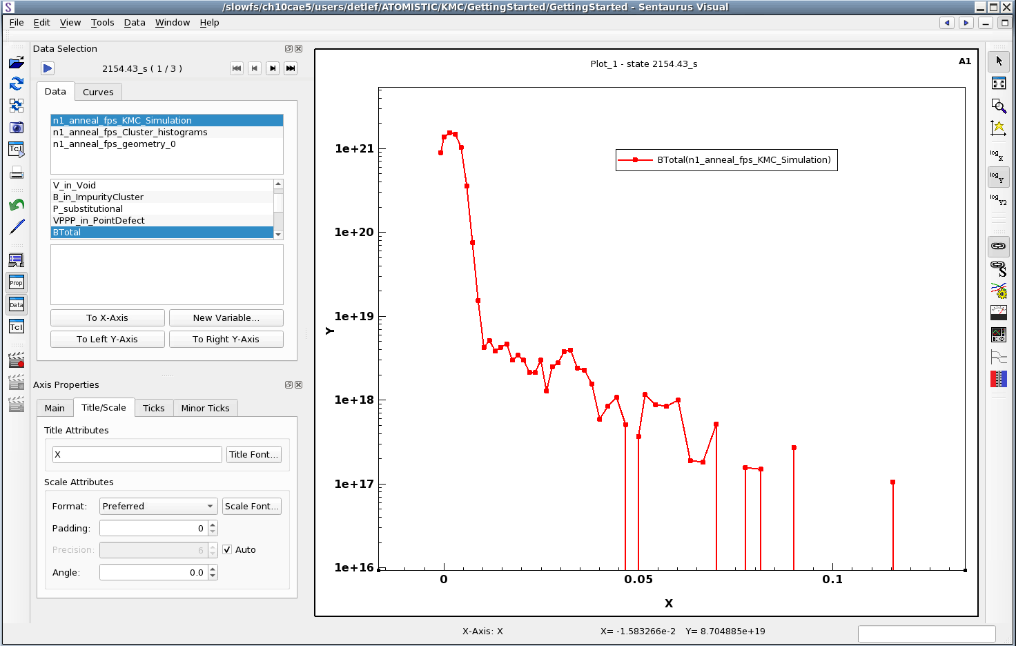
Figure 4. Dataset containing atomistic data written during the diffusion step. (Click image for full-size view.)
Figure 5 shows the second dataset, a cluster histogram, where the number of interstitial clusters versus cluster size is plotted. You see that, at the given instance, there are four clusters consisting of eight interstitials.
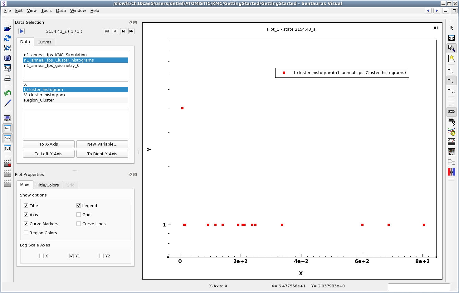
Figure 5. Dataset containing cluster histograms during the diffusion step. (Click image for full-size view.)
Figure 6 shows the n1_anneal_fps_Geometry_0 dataset that contains the atomistic information mapped onto the five-stream continuum diffusion model and the continuum mesh (see Figure 5). This dataset is written only at the end of the diffusion step.
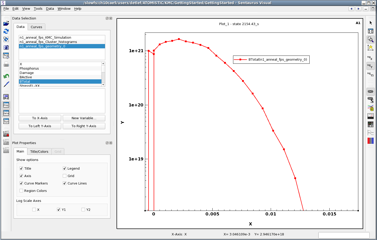
Figure 6. Dataset containing atomistic data mapped onto the five-stream model and continuum mesh. (Click image for full-size view.)
The second frame, labeled n1_anneal_fps_Dopants, shows the dopant–defect clusters BxIy and BxVy (see Figure 7). Such a plot is usually displayed best with the Convert to Nodal option switched off.
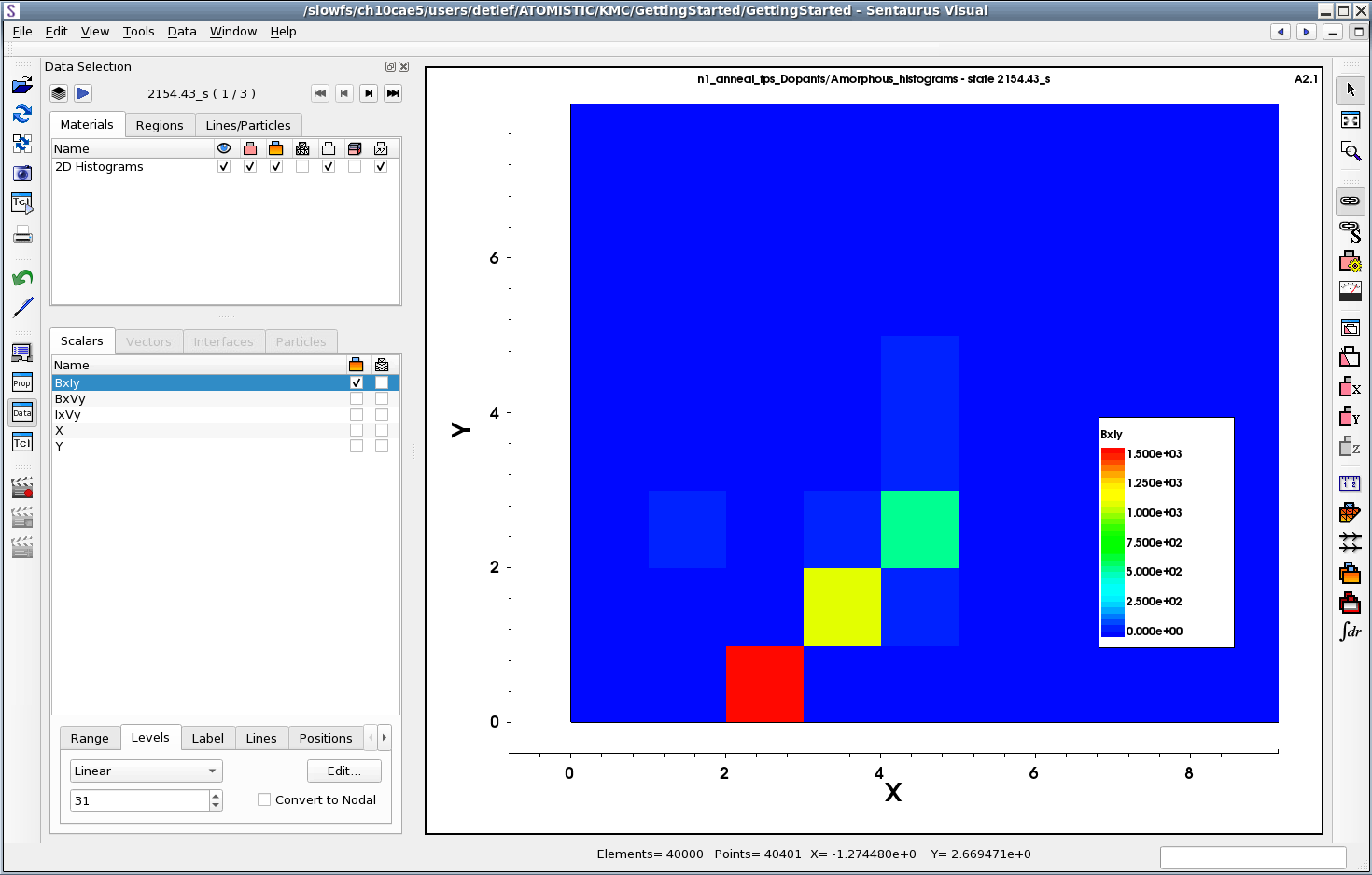
Figure 7. BxIy cluster distribution written during the diffusion step. (Click image for full-size view.)
The third frame, labeled n1_anneal_fps_KMC_Grid, shows individual dopants and defects. You can change how these are displayed using the Region Properties dialog box (see Figure 8).
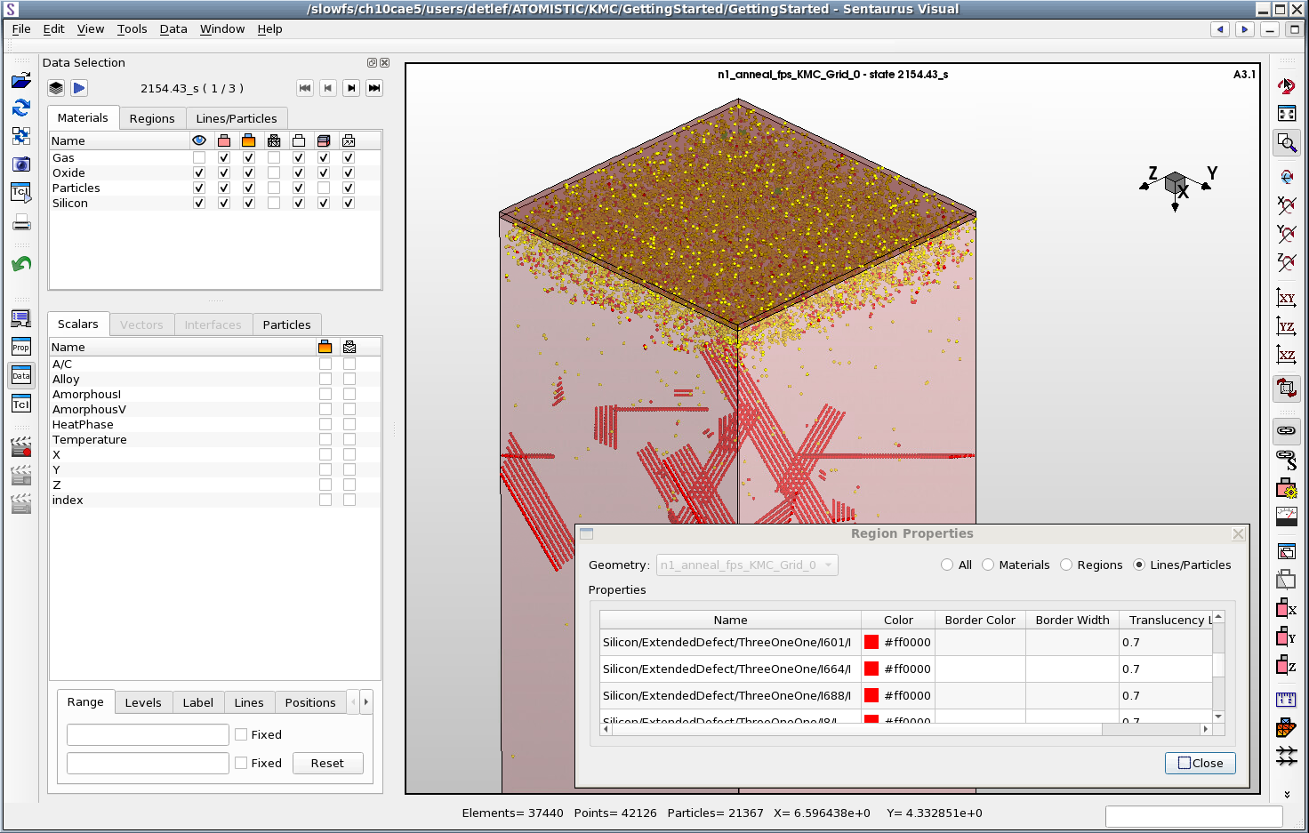
Figure 8. Snapshot showing all defects and dopants during the diffusion simulation. The Region Properties dialog box allows you to change the plot properties of defects. (Click image for full-size view.)
12.8 Understanding Information in the Log File
Sentaurus Process KMC prints a lot of information to the log file. Understanding this information is essential to understanding the results of an atomistic simulation.
First, the size of the KMC simulation domain and the continuum simulation domain are reported:
KMC domain (-0.1008, 0, 0) to (0.75, 0.04, 0.04) um Sentaurus domain (-0.1008, \
  0, 0) to (0.75, 0, 0) um.
The KMC simulation domain is usually as big as the structure plus the gas. For the lateral dimensions, the values that are defined either implicitly or explicitly are used and printed here (0.04 μm in the present example). This simulation domain is divided automatically into several KMC boxes, and Sentaurus Process KMC reports the number in each direction and the minimum and maximum box sizes:
KMC NonUniformTensor. Boxes: 37440
	X=117 (0.8 - 35.8459)nm (-100.8 - 750)
	Y=16 (2.5 - 2.5)nm (0 - 40)
	Z=20 (2 - 2)nm (0 - 40)
Second, a table with a summary of the models used is given:
| KMC models     | Germanium                                       |
+----------------+-------------------------------------------------+
|Interstitial    |                                                 |
|   DiffModel    |Direct(I)                                        |
|   ChargeModel  |I( -2 -1 0 1 2 )                                 |
|   ClusterModel |I+I AmorphousPocket Void ThreeOneOne Loop        |
|Vacancy         |                                                 |
|   DiffModel    |Direct(V)                                        |
|   ChargeModel  |V( -3 -2 -1 0 1 2 3 )                            |
|   ClusterModel |V+V AmorphousPocket Void ThreeOneOne Loop        |
|Boron           |                                                 |
|   DiffModel    |                                                 |
The table lists the diffusion model, possible charge states, the cluster model, and the model for solid phase epitaxial regrowth for all implemented impurities and for silicon and vacancies.
Third, the result of initializing the KMC simulation is printed:
Particle   Outside   Rejected    Created  (during atomizing Phosphorus)
P                 0          0          1 (Silicon)
A background concentration of 3.8e14 cm-3 phosphorus was specified. The size of the simulation domain allows then only one particle, which is created during the atomization process and is placed at a random position in silicon.
The next step in this example is the implantation of germanium. This process simulation step produces output such as:
KMC: Time(s)   Temp(C)       Events Events/s Average step(s)   %Done
2.154435e-01     26.85         1512                            0.02%
4.641589e-01     26.85         4900             7.341069e-05   0.04%
The table is self explanatory. The implantation occurred at room temperature, and the time was assumed to be 1000 s. The next table is a summary of particles that have been created during the implantation step:
Particle   Outside   Rejected    Created  (during implant)
I           0      0    4912456 (AmorphousSilicon)    1008314 (Silicon)
V           4     3930    4927471 (AmorphousSilicon)   988090 (Silicon)
Sii        1994    15786
KMC: During 'implant' Alloys were incorporated as a field and not as a particle
The last line is specific to the implantation of germanium. It states that Sentaurus Process KMC does not deal with individual Ge atoms after they are implanted, but germanium has been converted into a field (and, therefore, can be used for other purposes, such as stress calculation or in device simulations). In this table, Outside are particles that left the simulation domain by scattering processes. Rejected are particles that do not make sense in a certain material, such as anything in gas, or I and V in oxide.
In addition to this table, which is written after each implantation step, Sentaurus Process KMC produces several reports after each implantation step and each diffusion step:
- KMC particle distribution report
- KMC cluster distribution report
- KMC defect activity report
- KMC interactions report
- KMC event report
In the following, these reports are listed and briefly explained. See the Sentaurus™ Process User Guide for details. After the annealing, these reports look like the following ones:
--------------------- KMC Particle distribution report -----------------------
Material           Dopant   Total  State
AmorphousSilicon   B        13969    100.00% mobile
Oxide              B         1138    100.00% mobile
Silicon            B           11      0.00% active
This table lists the number of dopants in each material. In full materials (such as silicon), it states how many of the dopants are active (in substitutional places). In other materials (such as oxide), dopants are only mobile, that is, they are inactive and do not form clusters.
------------------  KMC impurity cluster distribution report -----------------
Name     #number
--- Silicon ---
BI2          4
This table lists all of the present impurity clusters. The next table – the activity report – lists all particles that were present in this part of the simulation. The list contains particles that still exist at the end of the simulation step, but it also lists particles that disappeared (for example, extended defects that dissolved during annealing). The report contains two columns with three subcolumns each. The first report shows when the model was first used; the last report shows when the model was last used. If the model is still being used, the number of particles or defects using it is displayed followed by here. The three subcolumns report the time, the number of simulated events, and the temperature.
In this particular example, the first positively charged interstitial was created after a time of 0.19 s at 27°C, and the last one was observed after 7206 s at 700°C.
------------------------- KMC defect activity report -------------------------
First:  Time Events   Temp |  Last: Time     Events Temp Label
       0.000 0.00e+00   27 |    43028 here               PointDefect (I)
       0.000 0.00e+00   27 |    42997 here               PointDefect (V)
       0.000 0.00e+00   27 |        1 here               PointDefect (P)
9.962816e-02 6.17e+02   27 |      1188.998 4.18e+06   27 PointDefect (IM)
5.779453e-01 6.94e+03   27 |      1165.162 4.16e+06   27 PointDefect (IP)
The next table is the interactions report. It lists all interactions in all materials that occurred during this part of the simulation. This table helps to understand which interactions are important. In this example, the interactions between neutral interstitials and between neutral interstitials and neutral vacancies dominate.
-------------------------- KMC interactions report ---------------------------
Object             Reaction    #Times  Reaction    #Times  Reaction    #Times

--- Silicon ---
PointDefect        I+I         126250  I+V         173622  I+P              3
The last report is the event report. The information in this report depends on the specified hopping mode. Here, the double mode was used. The report lists, for each mobile particle, the number of jumps in opposite directions, in the same direction, and in the orthogonal direction. For particles that can break up, the number of breakup events during the simulation is listed in the last column:
---------------------------  KMC event report   ------------------------------
--- Silicon ---

Name      Jump ><      Jump >>      Jump >^     Break-up     Percolat
PointDefect     I          358020       357905      1430272
PointDefect     V          170463       169371       675438
All these reports are written to the log file automatically. Of course, you can write more information to this file. For example, the following command counts the number of boron particles and prints this number to the log file:
LogFile "[kmc extract defects countparticles name= B ]"
12.9 Improving Resolution of Concentrations
From Section 12.5 Comparing Simulation Results to Measurements, it is clear that the resolution of the concentrations cannot be improved by making the mesh onto which the results are extracted finer and finer. The only way to improve the resolution is to increase the surface area.
You can estimate the minimum concentration that can be resolved with a certain surface area. Assuming a surface area of 32 nm x 32 nm and a continuum mesh spacing of 1 nm perpendicular to the surface, you see that one particle in such a thin slice represents a concentration of 1/1024 nm-3 = 1.0e18 cm-3. This means that concentrations below that cannot be resolved, because having or not having that particle in this slice means having concentrations of 1e18 or 0, respectively.
To illustrate this effect, the same example with surface areas of 0.01 μm2, 0.04 μm2, 0.1 μm2, and 0.15 μm2, corresponding to noise levels of 1e19 cm-3, 6.25e17 cm-3, 1.0e17 cm-3, and 4.4e16 cm-3, was simulated.
The peak of the boron concentration is represented well in all simulations (see Figure 9). Beyond the peak, however, it can be seen how each simulation reaches its noise level. The isolated lines at the right-hand side of the plot represent the effect of having only one particle in a slice or having none. Similarly, the limits of the resolution can be seen if you want to study the dynamics of extended defects. In Figure 10, the concentration of interstitials belonging to {311} defects is plotted. With the smallest surface area, this concentration cannot be resolved at all. With bigger surface areas, the resolution improves.
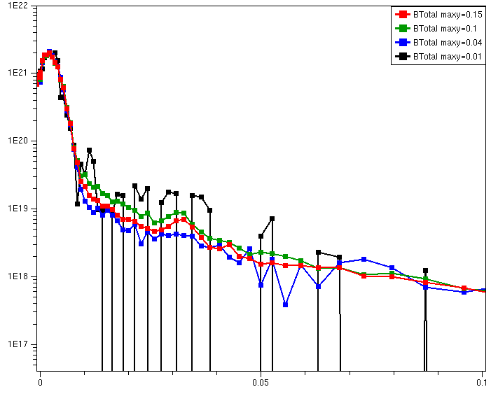
Figure 9. Total boron concentration after annealing. The colors indicate the surface area of the simulation domain. Black: 0.01 μm, blue: 0.04 μm, green: 0.1 μm, and red: 0.15 μm. The characteristic boron peak at 0.04 μm, which is seen experimentally, can be simulated only with larger simulation domains (green and red lines). (Click image for full-size view.)
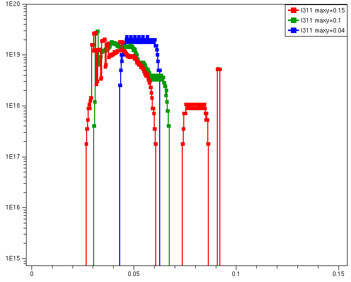
Figure 10. Interstitials belonging to {311} defects. The color code is the same as in Figure 9. The smaller simulation domain cannot resolve such a concentration. (Click image for full-size view.)
12.10 References
- Ref. 1
- R. Duffy et al., "Boron uphill diffusion during ultrashallow junction formation," Applied Physics Letters, vol. 82, no. 21, pp. 3647–3649, 2003.
- Ref. 2
- N. Zographos and I. Martin-Bragado, "A Comprehensive Atomistic Kinetic Monte Carlo Model for Amorphization/Recrystallization and its Effects on Dopants," in MRS Symposium Proceedings, Doping Engineering for Front-End Processing, vol. 1070, p. 1070-E03-01, March 2008.
Copyright © 2022 Synopsys, Inc. All rights reserved.