main menu | module menu | << previous section | next section >>

Sentaurus Mesh
2. Axis-Aligned Mesh Refinement

2.1 Basics
2.2 Refinement Regions
2.3 Refinement Controls
2.4 Multiboxes

Objectives

To introduce the axis-aligned mesh generation capabilities of Sentaurus Mesh.

2.1 Basics

In Sentaurus Mesh, the main mesh generation algorithm is the binary-tree decomposition to a device domain according to the command file specifications, followed by delaunization. The quadtree (2D) or octree (3D) recursive space decomposition technique used in Sentaurus Mesh discretizes a device domain that is combined with mesh delaunization (see Section 5.2 Mesh Delaunization).

Figure 1 illustrates the concept of quadtree space decomposition for a 2D device:

First, the quadrant (called root) is defined, which surrounds the entire device domain (in this case, it exactly matches the device boundary).
Second, the recursive split process starts when an entire domain is split into two subdomains in each direction, then each subdomain is again split into two subdomains, and so on, until the mesh spacing becomes less than or equal to the required mesh spacing.
Third, the entire domain is represented as a union of all leaf elements of the tree, from where it derives its name – the binary tree method.

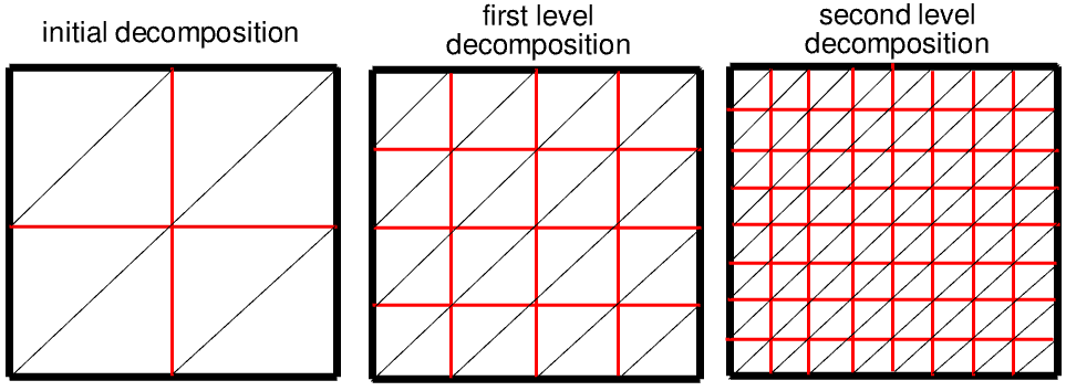
Figure 1. Illustration of the concept of quadtree space decomposition. (Click image for full-size view.)

Sentaurus Mesh requires that you supply a device boundary file. Furthermore, you must also create a command file where general mesh controls and optional doping specifications are defined. A command file can be created either manually (in a text editor) or using the corresponding Sentaurus Structure Editor functionality (see Section 4. Generating Meshes of the Sentaurus Structure Editor module).

The Sentaurus Mesh command files featured in this section are all contained in the Sentaurus Workbench project Applications_Library/GettingStarted/snmesh/Basics. Within this project, the preferences are selected such that Sentaurus Mesh will take the boundary file from the preceding Sentaurus Structure Editor tool instance, while the command file is created by a text editor (see Section 1.6 Sentaurus Mesh Integration in Sentaurus Workbench).

To work with the project, start Sentaurus Workbench and copy the project Basics to a local directory within your Sentaurus Workbench working directory to which the environment variable $STDB points. For details about this environment variable, see Section 1.2 Starting Sentaurus Workbench.

The features discussed in this section are demonstrated in the Sentaurus Mesh tool instance labeled test2d in this Sentaurus Workbench project.

A command file must include at least two independent sections. In the Definitions section, you specify mesh spacing controls (Refinement) and doping profiles, which then can be referenced in the Placements section.

First, you will mesh a piece of silicon material (2 μm x 2 μm).

Click to view the command file test2d_msh.cmd.

In this command file, only a single Refinement statement called "global" is declared, which specifies the maximum-allowed mesh element size as 0.5 μm in each of the spatial directions of the device. The "global" refinement is referenced in the Placements section under the same name without any position specification, indicating that the entire device will be meshed using the refinement specification in the Definitions section:

Definitions {
  Refinement "global" {
    MaxElementSize = (0.5 0.5)
  }
}
Placements {
  Refinement "global" {
    Reference="global"
  }
}

where the two values in the MaxElementSize specification indicate the maximal mesh step in the x- and y-direction.

For 2D device meshing, the value that corresponds to the third device dimension (usually, the z-coordinate) can be omitted.

Figure 2 shows the mesh generated by Sentaurus Mesh. Run the corresponding project node and view the generated mesh with Sentaurus Visual.

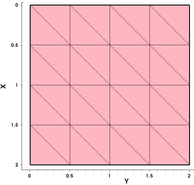
Figure 2. Mesh generated by Sentaurus Mesh. (Click image for full-size view.)

In Figure 2, you can see that the entire device first is decomposed into 16 rectangles (four in each direction), which then are triangulated. In this case, the edge length of each rectangle is 0.5 μm exactly, as specified in the refinement definition. The final mesh consists of 25 vertices and 32 elements.

For a similar (2 μm x 2 μm x 2 μm) 3D device structure and the command file test3d_msh.cmd, the final mesh consists of 125 vertices and 384 elements as shown in Figure 3.

Click to view the command file test3d_msh.cmd.

Run the project node of Sentaurus Mesh labeled test3d and view the generated mesh with Sentaurus Visual.

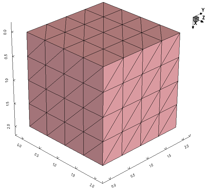
Figure 3. Three-dimensional device with 125 vertices and 384 elements. (Click image for full-size view.)

Having MaxElementSize control values not strictly proportional to the entire device dimensions results in a smaller element size than specified. For the above 2D device structure, the 0.4 μm maximal step value is specified in each direction:

Definitions {
  Refinement "global" {
    MaxElementSize = (0.4 0.4)
  }
}

With this setting, you might expect 2 μm/0.4 μm = 5 mesh steps in each direction. However, the binary-tree decomposition algorithm can produce only 2ⁿ mesh steps. So, you would have eight (8) steps in each direction (see Figure 4), which results in 128 mesh elements and 81 mesh vertices. This example makes it clear that, in most cases, the resulting mesh step will be lower than specified due to the restrictions of the binary-tree decomposition algorithm.

This behavior is exemplified in the project Basics at the Sentaurus Mesh tool instance labeled finerMesh. Run the corresponding project node and view the generated mesh with Sentaurus Visual.

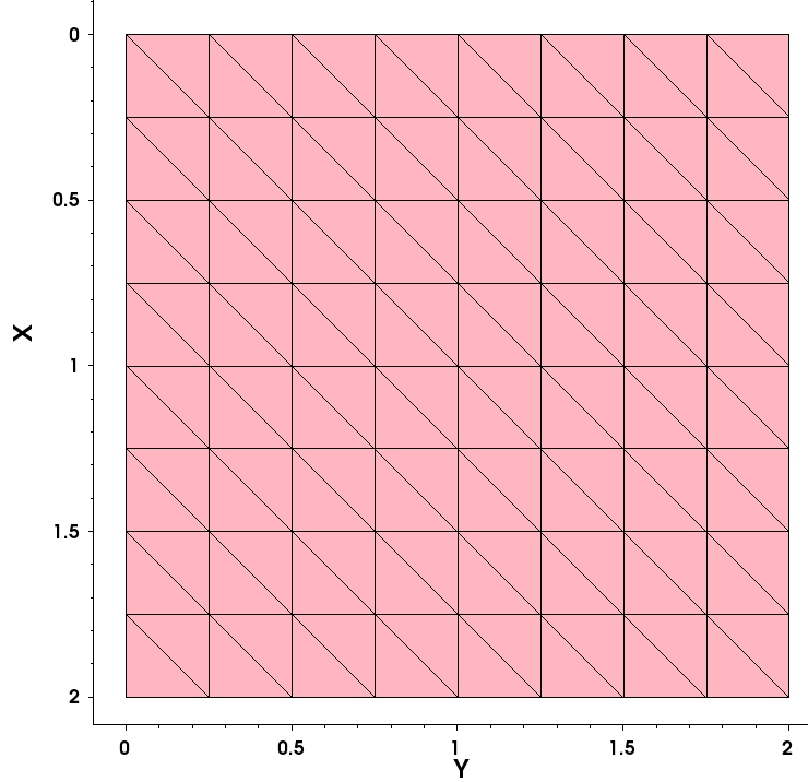
Figure 4. Two-dimensional mesh with smaller mesh steps. (Click image for full-size view.)

Now, you will see what happens with a nonaxis-aligned device. In this example, the device boundary used in the previous example is rotated 45°, and the same command settings as in the command file of the first example (rot2d_msh.cmd) are applied.

Click to view the command file rot2d_msh.cmd.

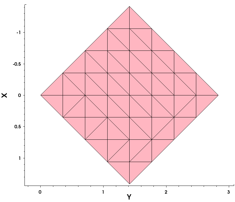
Figure 5. Two-dimensional mesh with smaller mesh steps, which is rotated 45°. (Click image for full-size view.)

As can be seen in Figure 5, for a rotated (nonaxis-aligned) structure, the binary-tree decomposition is applied to a larger domain, resulting in a larger number of mesh nodes. The final mesh consists of 78 elements and 55 vertices.

This behavior is exemplified in the project Basics at the Sentaurus Mesh tool instance labeled rot2d. Run the corresponding project node and view the generated mesh with Sentaurus Visual.

2.2 Refinement Regions

The Sentaurus Mesh command files featured in this section are all contained in the Sentaurus Workbench project Applications_Library/GettingStarted/snmesh/Refinements.

To work with the project, start Sentaurus Workbench and copy the project Refinements to a local directory within the Sentaurus Workbench working directory to which the environment variable $STDB points. For details about this environment variable, see Section 1.2 Starting Sentaurus Workbench.

As mentioned in Section 2.1 Basics, the refinement region is a geometric object, placed inside a device, which allows flexible control over a mesh step. The refinement region is represented by a geometric element, such as a rectangle, polygon, or complex polygon in the case of two dimensions, or a cuboid or polyhedron (the closed volume surrounded by multiple polygons) in the case of three dimensions. It also can refer to an entire material or region.

The syntax to define a refinement region in the Definitions section of the command file is:

Refinement "reference name" {
  MaxElementSize = (<xmax> <ymax> <zmax>)
  MinElementSize = (<xmin> <ymin> <zmin>)
  RefineFunction = MaxGradient(parameters) | MaxInterval(parameters) | 
                   MaxTransDifference(parameters) | 
                   MaxLengthInterface(parameters)
}

where:

MaxElementSize and MinElementSize indicate the maximum-allowed and minimum-allowed mesh step values inside a refinement region along a particular axis.
RefineFunction specifies the mesh refinement controls (see Section 2.3 Refinement Controls).
MaxLengthInterface activates mesh refinement at interfaces (see Section 3.2 Interface Refinement).

The corresponding refinement instance definition in the Placements section is:

Placements {
  Refinement "instance name" {
    Reference = "string"
    RefineWindow = geometric element | material | region
  }
}

For multiple refinement specifications, the refinement regions can overlap. If this is the case, a refinement region with the smallest step definition "wins".

The following example demonstrates this, with the rectangular refinement region inside the test device structure with smaller step definitions compared to the global ones:

Definitions {
  Refinement "global" {
    MaxElementSize = (0.5 0.5 0.5)
  }
  Refinement "rectangle" {
    MaxElementSize = (0.125 0.125 0.125)
  }
}

Placements {
  Refinement "global" {
    Reference="global"
  }
  Refinement "rectangle" {
    Reference = "rectangle"
    RefineWindow = Rectangle [(0.75 0.75) (1.25 1.25)]
  }
}

The resulting mesh is shown in Figure 6, where the contour of the rectangular refinement region is highlighted. The transition from the finer mesh inside the rectangular refinement to the coarser mesh outside the region, due to mesh smoothing, is clearly seen (see Section 5.1 Mesh Smoothing).

This behavior is exemplified in the project Refinements at the Sentaurus Mesh tool instance labeled rectangle. Run the corresponding project node and view the generated mesh with Sentaurus Visual.

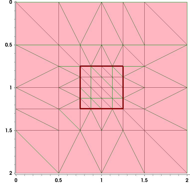
Figure 6. Rectangular 2D refinement. (Click image for full-size view.)

The next example demonstrates the regionwise refinement approach, where the polygonal region called PolygonR is introduced inside the device test structure.

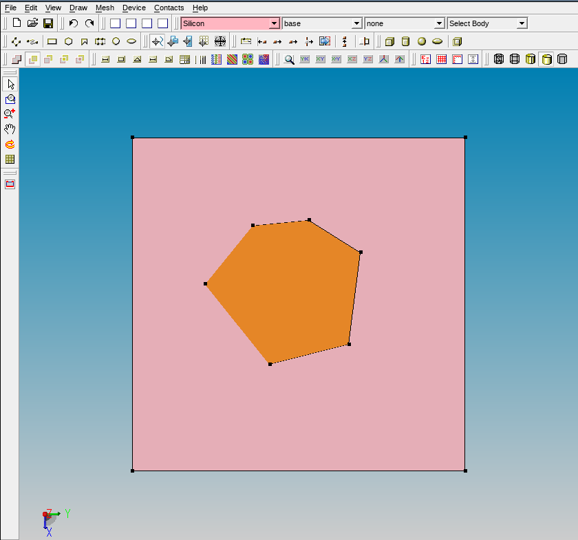
Figure 7. Polygonal region inside device structure shown in Sentaurus Structure Editor. (Click image for full-size view.)

Different refinement criteria are used inside and outside the polygonal region refinement. Inside the polygonal region, a smaller mesh step is specified, compared to the global step definition:

Definitions {
  Refinement "global" {
    MaxElementSize = (0.5 0.5 0.5)
  }
  Refinement "polygon" {
    MaxElementSize = (0.25 0.25 0.25)
  }
}

To confine the mesh refinement inside the polygonal region, the regionwise refinement placement is defined using the RefineWindow specification:

Placements {
  Refinement "global" {
    Reference="global"
  }
  Refinement "polygon" {
    Reference = "polygon"
    RefineWindow = region ["PolygonR"]
  }
}

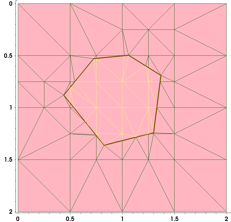
Figure 8. Polygonal mesh refinement. (Click image for full-size view.)

This behavior is exemplified in the project Refinements at the Sentaurus Mesh tool instance labeled polygon. Run the corresponding project node and view the generated mesh with Sentaurus Visual.

Different mesh colors help to visualize the transition from denser to coarser mesh areas.

The next example demonstrates how materialwise mesh refinement is performed. In this example, two adjacent materials, silicon and oxide, are meshed with different mesh steps (0.5 μm in silicon and 0.125 μm in oxide):

Definitions {
  Refinement "Si" {
    MaxElementSize = (0.5 0.5 0.5)
  }
  Refinement "Ox" {
    MaxElementSize = (0.125 0.125 0.125)
  }
}

Placements {
  Refinement "Si" {
    Reference = "Si"
    RefineWindow = material ["Silicon"]
  }
  Refinement "Ox" {
    Reference = "Ox"
    RefineWindow = material ["Oxide"]
  }
}

Figure 9 shows the resulting mesh. The smaller mesh step propagates from the silicon–oxide material interface towards silicon because of the applied mesh smoothing (see Section 5.1 Mesh Smoothing).

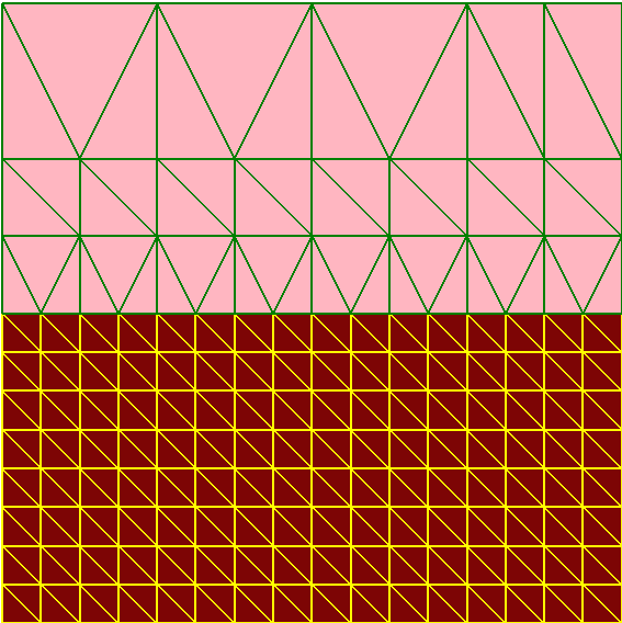
Figure 9. Materialwise mesh refinement. (Click image for full-size view.)

This behavior is exemplified in the project Refinements at the Sentaurus Mesh tool instance labeled materials. Run the corresponding project node and view the generated mesh with Sentaurus Visual.

2.3 Refinement Controls

One of the major features of Sentaurus Mesh is automatic mesh refinement, which allows you to accurately resolve areas with geometry or profile spatial nonuniformities. This section discusses the mesh refinement of a nonuniform doping distribution.

The Sentaurus Mesh command files featured in this section are all contained in the Sentaurus Workbench project Applications_Library/GettingStarted/snmesh/RefineControls.

To work with the project, start Sentaurus Workbench and copy the project RefineControls to a local directory. The target directory must reside under the Sentaurus Workbench working directory to which the environment variable $STDB points. For details about this environment variable, see Section 1.2 Starting Sentaurus Workbench.

The following example demonstrates automatic mesh refinement on doping for a 2D p-n junction device structure. The automatic refinement procedure uses the RefineFunction specification inside a Refinement section. The resulting doping profile is a combination of the uniformly distributed boron doping and nonuniformly distributed phosphorus doping (see Figure 10).

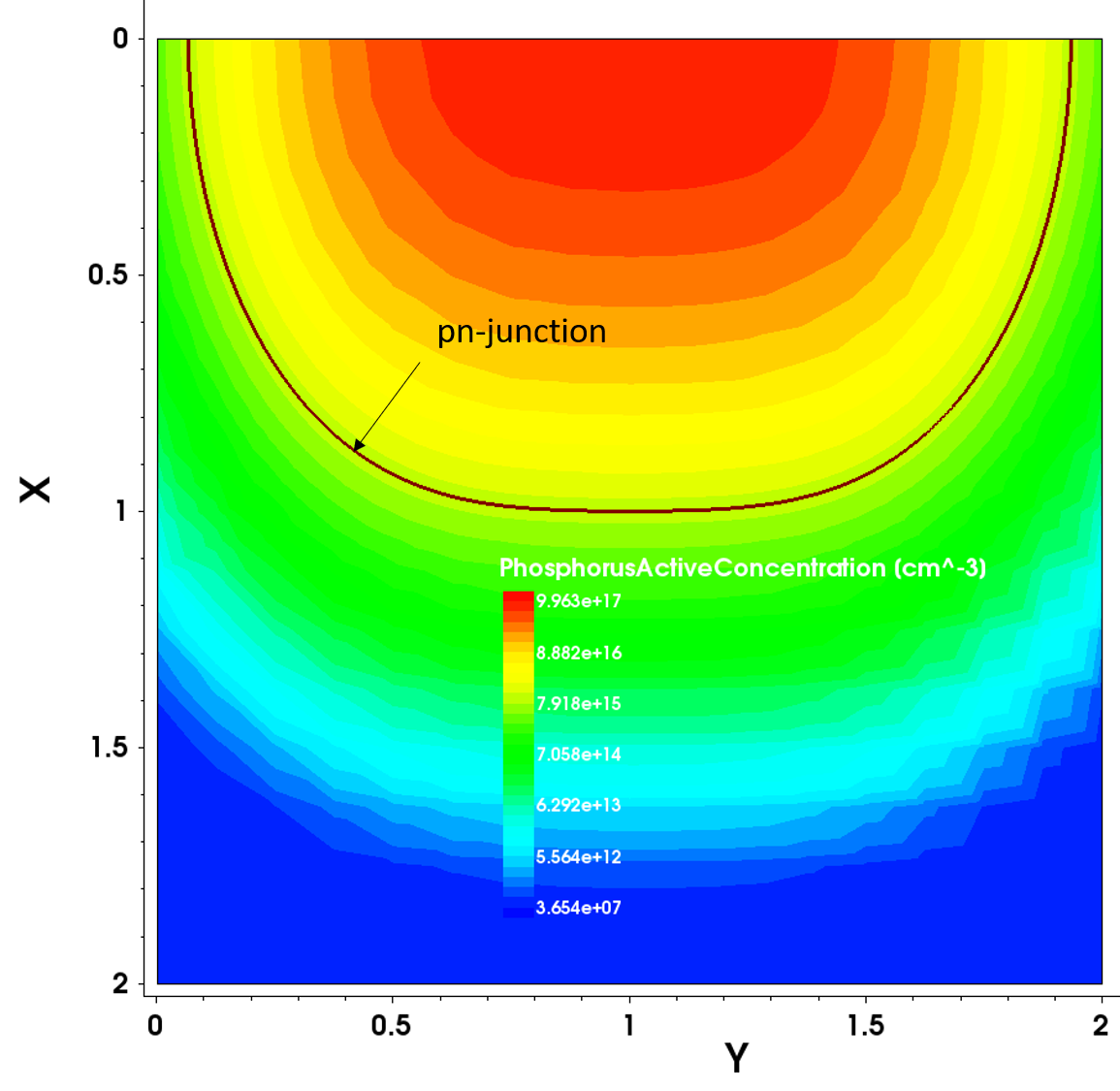
Figure 10. Two-dimensional phosphorus distribution. (Click image for full-size view.)

Various settings discussed in this section are selected in the project RefineControls by the Sentaurus Workbench parameters @DopRefType@ and @Value@.

For @DopRefType@ set to None, the mesh is generated without having a RefinementFunction specification included in the global Refinement section of the command file (the doping definition used in the command file is discussed in Section 4. Doping Definition):

Definitions { ...
  Refinement "global" {
    MaxElementSize = ( 0.2 0.2 0.2 )
    MinElementSize = ( 0.01 0.01 0.01 )
  }
}

...

Placements { ...
  Refinement "global" {
    Reference = "global"
    RefineWindow = material ["Silicon"]
  }
}

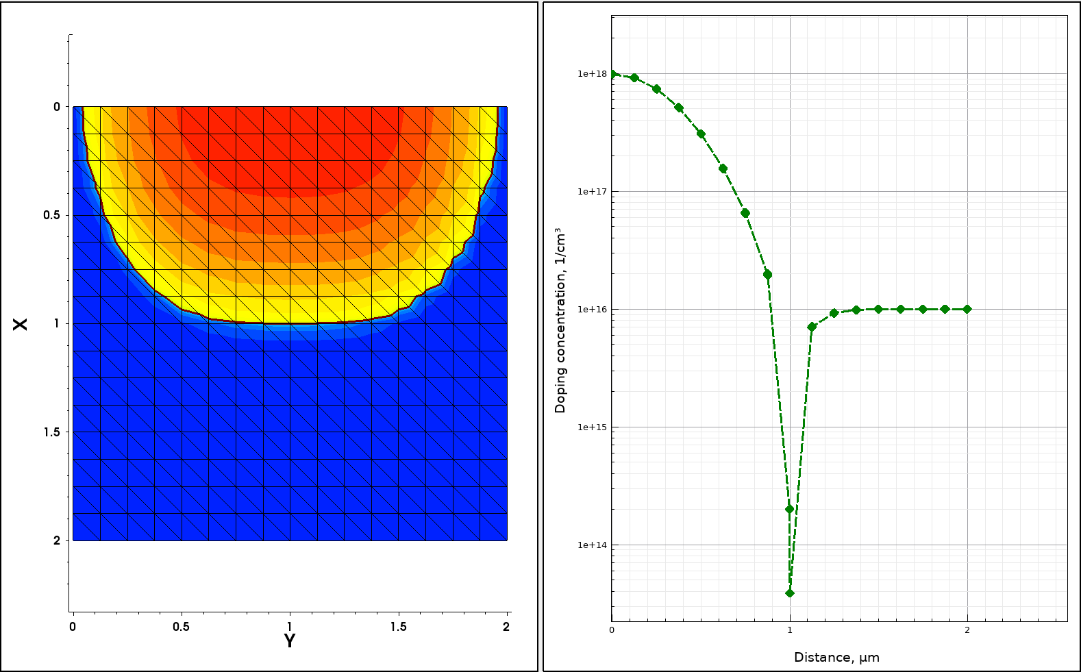
Figure 11. (Left) Two-dimensional uniform mesh and resulting doping profile distribution and (right) resulting doping profile on a uniform mesh, cut at x=1 coordinate across the p-n junction. (Click image for full-size view.)

As can be seen, the nonuniform part of the resulting doping profile is covered by only nine mesh steps in the vertical direction, which is not sufficient to accurately resolve the profile spatial nonuniformity. In the end, such a coarse mesh will cause inaccurate results from the device electrical simulation perspective and can lead to simulator failure.

For @DopRefType@ set to MaxTransDiff and @Value@ set to 1, the mesh is generated with an additional RefinementFunction statement in the Refinement description:

Definitions { ...
  Refinement "global" {
    MaxElementSize = ( 0.2 0.2 0.2 )
    MinElementSize = ( 0.01 0.01 0.01 )

    RefineFunction = MaxTransDiff(Variable="DopingConcentration", Value=@Value@)

}
}

The MinElementSize parameter specifies the lower bound for the edge size of the mesh element in each spatial direction. These values are used for automatic mesh refinement on the doping. The RefineFunction statement activates the automatic mesh refinement based on the provided specification. In this particular case, the automatic refinement is based on the value difference of the resulting doping concentration. The keyword MaxTransDiff indicates that the hyperbolic arcsine function (asinh) should be used for the mesh refinement on doping.

The mesh refinement algorithm checks whether a function value difference between two neighboring mesh points is greater than a specified value (Value=1 in this case) and then refines the mesh accordingly.

Figure 12 shows the resulting mesh doping refinement, which was obtained with the above specification.

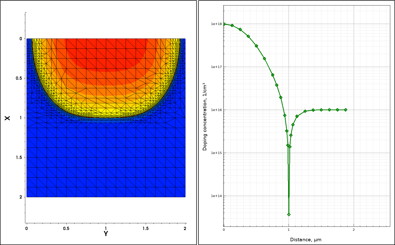
Figure 12. (Left) Two-dimensional mesh refinement on doping, showing the fine mesh resolution within the p-n junction area and (right) resulting doping profile cut at x=1 coordinate across the p-n junction, and the steep doping gradient is now much better resolved. (Click image for full-size view.)

Run the RefineControls project and view the generated mesh at the corresponding node with Sentaurus Visual.

As an alternative to the asinh (MaxTransDiff) function, the gradient of the function can be used as a refinement function. In this project, this is done for @DopRefType@ set to MaxGradient and @Value@ set to 1 (or 10). In this case, the mesh is generated with an additional RefinementFunction statement in the Refinement description:

Definitions { ...
  Refinement "global" {
    MaxElementSize = ( 0.2 0.2 0.2 )
    MinElementSize = ( 0.01 0.01 0.01 )

    RefineFunction = MaxGradient(Variable="DopingConcentration", Value=@Value@)

}
}

If the gradient is greater than a specified value and the edge length is large enough, the element is refined. Figure 13 compares two meshes that were constructed with the MaxGradient doping refinement option using two different gradient values, namely, 1 and 10.

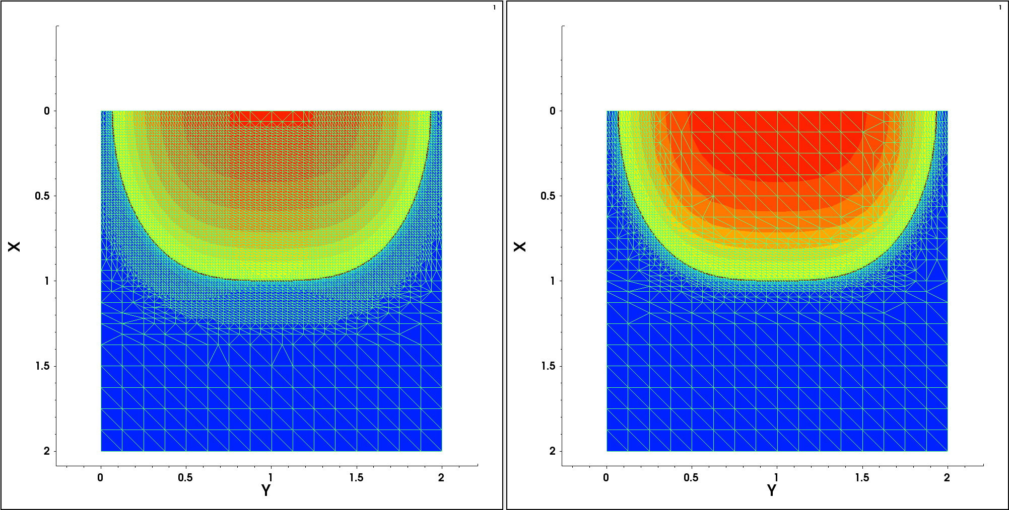
Figure 13. Refinement with (left) Value=1 and (right) Value=10. (Click image for full-size view.)

Another available option is to restrict the refinement to a certain range of values of a specific variable. In this project, this is done for @DopRefType@ set to MaxInterval. In this case, the mesh is generated with a different RefinementFunction statement in the Refinement description:

    RefineFunction = MaxInterval(Variable = "DopingConcentration", 
    	cmin = 1e16, cmax = 1e17, targetLength = 0.01
    )

The MaxInterval function analyzes each edge in a refinement tree cell and refines the edge if the data values are within the interval defined by cmin and cmax and the edge is longer than the targetLength.

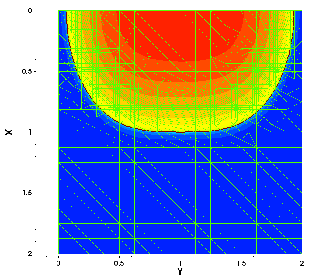
Figure 14. Interval refinement. (Click image for full-size view.)

The refinement method used in Sentaurus Mesh is based on the binary tree, where each edge is split in two along a given direction until either a MinElementSize is fulfilled or required element aspect ratio criteria are fulfilled.

2.4 Multiboxes

Another method to define mesh refinement is a multibox, which is a special refinement box that is used to specify an isotropically graded refinement along one of the x-direction, y-direction, or z-direction.

Using multiboxes is not recommended. In general, interface refinement (see Section 3.2 Interface Refinement) or offsetting (see Section 3.3 Offsetting) is easier than defining multibox refinement.

The syntax to define a multibox refinement in the Definitions section of the command file is:

Multibox "multibox reference name" {
  MaxElementSize = (<xmax> <ymax> <zmax>)
  MinElementSize = (<xmin> <ymin> <zmin>)
  Ratio = (ratio_x ratio_y ratio_z)
}

where:

MaxElementSize and MinElementSize are the same step definitions as for the refinement region.
Ratio controls the grading of the element size along each axis direction.

A simple example that demonstrates the use of a multibox to generate a gradual mesh is given in the project Refinements (see Section 2.2 Refinement Regions) at the Sentaurus Mesh tool instance labeled multibox1. It uses the same 2 μm x 2 μm silicon block device boundary as in the previous examples. Run the corresponding project node and view the generated mesh with Sentaurus Visual.

Definitions {
  Multibox "mb" {
    MaxElementSize = (1 1)
    MinElementSize = (0.1 0.1)
    Ratio = (2 1)
  }
}
Placements {
  Multibox "mb" {
    Reference = "mb"
    RefineWindow = rectangle[(0 0) (2 2)]
  }
}

Grading factors specified in the Ratio parameter control the gradual meshing in the corresponding direction. Having a grading factor higher than 1 (or lower than –1) means that the initial mesh step value, which is defined as MinElementSize, is used in the corresponding direction (in the above example, it is the y-direction). Each subsequent mesh step calculation is based on the formula step(i)=step(i-1)*ratio_factor.

If a ratio factor equals 1 exactly, grading is not produced, but the MaxElementSize step value is used instead. If a ratio factor equals 0 exactly, the corresponding specification is ignored. The mesh produced with the above specification is shown in Figure 15.

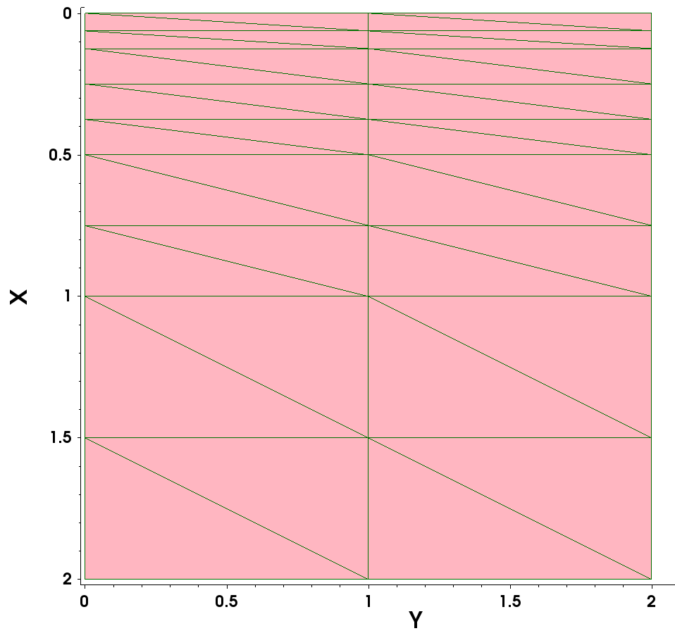
Figure 15. Mesh produced with multibox specification. (Click image for full-size view.)

As you can see, the mesh grading is produced along the y-direction from the top to the bottom, following the multibox Ratio specification. The initial step value produced in this example differs from the specified one (it is smaller than 0.1 μm). This is again a result of the specifications of the binary-tree decomposition algorithm (see Section 2.2 Refinement Regions).

The next example demonstrates how you can use a negative grading ratio value to control the grading direction. The following changes were made to the multibox definition in the command file:

Definitions {
  Multibox "mb" {
    MaxElementSize = (1 1)
    MinElementSize = (0.1 0.1)
    Ratio = (2 -2)
  }
}

Having a y-axis ratio factor equal to –2 means that Sentaurus Mesh will change the grading direction from downwards to upwards. In addition, note how gradings in different directions can be combined. Arrows indicate the corresponding multibox grading directions (see Figure 16).

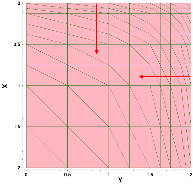
Figure 16. Multibox direction controls. (Click image for full-size view.)

A demonstration of the use of multiboxes to generate gradings in different directions is given in the project Refinements (see Section 2.2 Refinement Regions) at the Sentaurus Mesh tool instance labeled multibox2. Run the corresponding project node and view the generated mesh with Sentaurus Visual.