main menu | module menu | << previous section | next section >>

Sentaurus Interconnect
3. Example: Cantilever With End Load (3D)

3.1 Overview
3.2 Creating the 3D Structure and Its Mesh
3.3 Defining the Elastic Moduli of the Material
3.4 Setting the Boundary Conditions and Loads for the Solution
3.5 Solving the Problem
3.6 Postprocessing the Results
3.7 Using Second-Order Elements

Objectives

To perform a 3D mechanics simulation of a cantilever with an end load.

3.1 Overview

In this example, Sentaurus Interconnect will solve a simple case of a cantilever with an end load (see Figure 1). The cantilever is fully clamped at one end, and a point force is applied to the other end. No other loads or boundary conditions (BCs) are applied, and the entire structure is free to move under the effect of the applied force (except, of course, the clamped end).

The cantilever is expected to bend slightly on the xz plane with a maximum displacement \(δ_{\text"max"}\) at the end where the point force is applied, which is given by the analytic model (valid only for small displacements, that is, the linear regime):

\[δ_{\text"max"} = 4 {P L^{3}} / {E α^4} \]

where \(E\) is Young's modulus, \(P\) is the point force, \(L\) is the length of the cantilever, and \(α\) is the edge of the square cross-section of the cantilever.

The complete project can be investigated from within Sentaurus Workbench in the directory Applications_Library/GettingStarted/sinterconnect/3D_Cantilever.

Figure 1. Cantilever 3D structure with an end load and the other end fully clamped. (Click image for full-size view.)

3.2 Creating the 3D Structure and Its Mesh

In this section, you define the 3D structure of the cantilever and the meshing. The cantilever has a 4×4 μm² square cross-section and is 50 μm long (set by the Sentaurus Workbench parameter @1@). This is performed using line commands to define the boundaries of the structure in the three basic directions: x, y, and z.

The main axis of the cantilever is oriented parallel to the x-axis with the center of its cross section along the line y=0 z=0. The initial meshing of the structure is achieved by specifying spacing=<n> of the line command. The exact placement of the lines is done by location=<n>, and the default unit is μm. Tags can be used to identify the lines of interest by specifying tag=<c>.

These tags are not related in any way to the tags used later to set the BCs.

Finally, the grid definition section looks like this:

line x location= 0.0<um>  spacing= @res@<um>   tag= top
line x location= @l@<um>  spacing= @res@<um>   tag= bottom
line y location= -2.0<um> spacing= @res@<um>   tag= left
line y location= 0.0<um>  spacing= @res@<um>
line y location= 2.0<um>  spacing= @res@<um>   tag= right
line z location= -2.0<um> spacing= @res@<um>   tag= back
line z location= 0.0<um>  spacing= @res@<um>
line z location= 2.0<um>  spacing= @res@<um>   tag= front

The Sentaurus Workbench parameter @res@ sets the global spacing of the grid, and the default value in the project is 0.3 μm. This spacing value can be changed slightly up or down, depending on the global size of the simulation domain and the initial grid division by Sentaurus Mesh. Figure 2 shows the meshed 3D model along with the orientation of the coordinate system.

Figure 2. Cantilever 3D structure with mesh. (Click image for full-size image.)

3.2.1 Defining the Simulation Domain

Before proceeding to the next steps, the simulation domain must be defined and initialized in Sentaurus Interconnect. All the initial regions must be set using the already existing tagged coordinates in the grid. In this case, only one region is present that you define using the region command. The material has been chosen to be silicon, but other materials in the parameter database can be used as well:

region silicon substrate xlo= top xhi= bottom ylo= left yhi= right zlo= back \
  zhi= front

To obtain a complete list of all the materials in the parameter database, use the command mater list.all on the command line. After the region settings, you must initialize the simulation domain with the init command:

init !DelayFullD

The option !DelayFullD is used so that Sentaurus Interconnect considers the full 3D space from the beginning. By default, as in Sentaurus Process, the initial domain is always 1D until a process step forces the simulator to add a dimension (for example, by using a mask). For more details, refer to the Sentaurus Process module, Section 3.2 Defining the Initial 2D Grid and Simulation Domain, or the Sentaurus™ Interconnect User Guide.

3.2.2 Saving the Initial Model

The initialized structure can be saved before proceeding to the next steps with the struct command and the tdr=<c> argument:

struct tdr=n@node@_init

In order for the saved file to be available in Sentaurus Workbench for visualization, the file name contains the running-node parameter @node@.

3.3 Defining the Elastic Moduli of the Material

The material properties for silicon are already set in the Sentaurus Interconnect database and, in general, there would be no need to define them. If you need to modify these properties, use the command pdbSet followed by the necessary options.

In this example, the bulk and shear moduli of the chosen material are changed to some arbitrary values by setting the Young's modulus and the Poisson ratio equal to 1 GPa (=10¹⁰ dyn/cm²) and 0.2, respectively. The conversion to the bulk and shear moduli is performed with the built-in Tcl functions Enu2K and Enu2G:

pdbSet Silicon Mechanics BulkModulus [Enu2K 1e10 0.2]
pdbSet Silicon Mechanics ShearModulus [Enu2G 1e10 0.2]

Internally, the Sentaurus Interconnect database always uses the units dyn/cm² for pressure and cm for lengths.

3.4 Setting the Boundary Conditions and Loads for the Solution

The last important step before the solution is to set all the boundary conditions (BCs) and loads. The general command for setting the BCs or loads is stressdata followed by the bc.location and bc.value arguments:

stressdata bc.location=Bottom bc.value= {dx=0 dy=0 dz=0}
stressdata bc.location=Left bc.value= {sx=0 sy=0 sz=0}
stressdata bc.location=Right bc.value= {sx=0 sy=0 sz=0}
stressdata bc.location=Back bc.value= {sx=0 sy=0 sz=0}
stressdata bc.location=Front bc.value= {sx=0 sy=0 sz=0}
stressdata bc.location=pointend point.coord= {0 0 0} bc.value= {pfx=0 pfy=0 \
  pfz=@p@<dyn>}

The default BC tags assigned to the five uppermost surfaces of the 3D simulation domain in Sentaurus Interconnect are Bottom, Left, Right, Back, and Front. There is no "Top" tag for the upper surface.

To constrain the displacements and rotations in the three directions xyz at the bottom of the cantilever (at x=50 μm), set all velocities to zero by specifying bc.location=Bottom and bc.value= {dx=0 dy=0 dz=0} (dx, dy, dz are in cm/s with the denominator /dt being assumed).

The four lateral surfaces (Left, Right, Back, and Front) of the cantilever should not be constrained with any force or displacement restriction and, therefore, zero stresses are applied in all directions with bc.value= {sx=0 sy=0 sz=0} in the stressdata command.

The point force is applied by specifying the coordinates of the application point with point.coord= {0 0 0} and the orientation and value of the force. The latter is done with bc.value= {pfx=0 pfy=0 pfz=@p@<dyn>}, where pfx, pfy, and pfz are the point forces along the x-, y-, and z-axes, respectively. During the solution, the nearest mesh node to the defined point will be selected to apply the force. The tolerance of this selection can be controlled by the following command:

pdbSet Mechanics Point.Snap.Dist <n>

The default value of this tolerance is 1 nm. If you activate the moving mesh option in Sentaurus Interconnect, an additional option must be activated to force the application point to follow the mesh updates:

pdbSetBoolean Mechanics Point.Force.Snap 1

In this example, the mesh remains static for simplicity and this does not affect the accuracy of the results. During postprocessing, a deformed version of the structure can be saved by applying all the calculated displacements to the structure. For more information about the moving mesh, refer to the Sentaurus™ Interconnect User Guide.

3.5 Solving the Problem

When all the BCs and loads are defined, you continue with the solution of the problem. In Sentaurus Interconnect, it is important to specify the mode of the simulation as there are many physical domains that can be simulated (for example, mechanical, electrical, and thermal) alone or combined. For this problem, the mechanical domain is of interest and is set with the mode command before the solve command:

mode mechanics
solve

With solve, the simulator assembles the system matrix and solves the problem using the default iterative linear solver (ILS) at the default temperature of 26.85°C. More information about the solvers supported in Sentaurus Interconnect can be found in the Sentaurus™ Interconnect User Guide.

3.6 Postprocessing the Results

When the solution is completed, you can inspect the results and extract the values of interest. In the case of a mechanics problem, the strains, the stresses, and the displacements are of interest. In general, you can visualize the entire 3D model with the results mapped on it by saving the structure in TDR format:

struct tdr=n@node@
struct tdr=n@node@_def deform deform.scale= 5.0

As previously mentioned, you can save the deformed structure in a TDR file using the deform option of the struct command. Another argument deform.scale=<n> can be added if you want to scale the displacement field for easier visualization. In this case, a factor of 5 is used for scaling. The TDR files can be visualized using Sentaurus Visual.

In Figure 3, the displacements in the z-direction as well as the strains and stresses along the x-axis are shown on the deformed structure. You can clearly see that the displacement is highest at the tip of the cantilever where the force is applied, as expected. The calculated value for the maximum displacement is approximately equal to 0.58 μm, very close to the value given by the analytic formula (0.586 μm).

Figure 3. Visualization of (left) displacements in z-direction shown on deformed cantilever, (middle) strains in x-direction on deformed structure, and (right) stresses in x-direction mapped onto deformed structure. (Click image for full-size view.)

It is also possible to control the visualization from a script by selecting the calculated field to be plotted. This is done with the select command followed by the definition of the field z="<field>". You can list all the calculated fields in the TDR file using the select command with the option list.all on the command line, provided that the TDR file containing the result is loaded beforehand with the command init tdr=<c>.

For the fields that are tensors of rank one or higher (for example, vectors and stresses), you can add an underscore and then the index of the tensor element you need as a suffix. For example, for the displacement in the x-direction, use z="Displacement_x" or, for the stress normal to the yz plane, z="Stress_xx" (nodal solution) or z="StressEL_xx" (element solution).

With the field of interest selected, you can create a plot of it along a certain line, as it is done in this project with the plot.1d command:

select z="Displacement_z"
plot.1d y=0 z=0

When the plot.1d command is executed, a window displaying the plot opens as shown in Figure 4. Remember that if you launch Sentaurus Interconnect from Sentaurus Workbench, Sentaurus Interconnect must be set to the interactive mode in order for this window to open.

Other options for plotting and saving the results are available using either the command line or a script, as well as from Sentaurus Visual. For more information about plot commands (for example, plot.1d, plot.2d), refer to the Sentaurus™ Interconnect User Guide.

Figure 4. Plot of the displacements (cm) in the z-direction along the longitudinal axis (y=0 z=0) of the cantilever using the plot.1d command. (Click image for full-size view.)

3.7 Using Second-Order Elements

So far, you have used a relatively dense mesh to obtain enough accuracy in the results. The elements used in the previous part are first-order (linear) elements. In that case, only the corner nodes of each element contain information on displacements and deformation, and the stresses in the element have a constant value.

If second-order (quadratic) elements are used, the centers of all the element edges also contain solution information, and the stresses within the element can vary. This means that the accuracy of the solution is better when second-order elements are used, and this can be achieved with a coarser mesh with respect to a model meshed with first-order elements.

To use second-order elements in Sentaurus Interconnect, use the command:

pdbSetDouble Mechanics FiniteElementOrder 2

It is easy to verify the efficiency of second-order elements in your project. You can set the Sentaurus Workbench parameter @res@=3.0, that is, a 10 times larger element size for the mesh, with and without using second-order elements (that is, add or remove, respectively, pdbSetDouble Mechanics FiniteElementOrder 2 in the script).

In Figure 5, you can see the significant error in the calculated displacements when using first-order elements with such a coarse mesh. In contrast, in Figure 6, the accuracy is unaffected and remains the same as in Figure 4 where a 10-times smaller element size was used.

The small cost when using second-order elements is that the execution time is longer compared to the solution of the same problem (same mesh density) with first-order elements. Sometimes, convergence takes longer to achieve with quadratic elements compared to linear elements, but this also depends on the problem to be solved.

There are many problems in which the mesh must be very dense to obtain an accurate solution with first-order elements, but they can be very expensive in terms of memory usage and execution time. These problems can benefit from using second-order elements in terms of both memory and execution time by preserving the same level of accuracy as for the fine-meshed models.

In Sentaurus Interconnect, second-order elements can be used with the elasticity and plasticity models only.

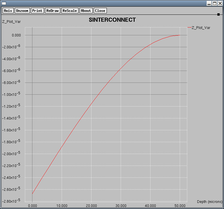
Figure 5. Plot of the displacements (cm) in the z-direction along the longitudinal axis (y=0 z=0) of the cantilever using first-order elements with an element size of 3.0 μm. The accuracy of the result is poor compared to Figure 4 and the analytic solution. (Click image for full-size view.)

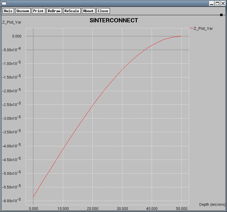
Figure 6. Plot of the displacements (cm) in the z-direction along the longitudinal axis (y=0 z=0) of the cantilever using second-order elements and the same element size as in Figure 5. The accuracy of the result is the same as in Figure 4, where a 10-times smaller mesh cell has been used with first-order elements. (Click image for full-size view.)