
Sentaurus Device
6. Nonlinear System Newton Solver
6.1 Solving Nonlinear Equation System With Newton Solver
6.2 Achieving a Good Initial Guess
6.3 Optimizing the Nonlinear Solver Performance
6.4 Using the Extrapolate Option
6.5 Determining the Convergence of the Newton Solver
6.6 Improving Convergence in Low-Density or Low-Current Regions
6.7 Debugging Newton Solver–Related Convergence Issues
Objectives
- To provide guidelines for selecting the most appropriate Newton solver settings in Sentaurus Device.
6.1 Solving Nonlinear Equation System With Newton Solver
Specifying the Coupled command in the Solve section of a Sentaurus Device tool input file activates the Newton-like solver over a set of equations. Available equations include the Poisson and continuity equations, as well as the heat and the energy transport equations:
Coupled ( <optional parameter> ){ <set of equations> }
To solve the transport model equations self-consistently, Sentaurus Device uses the iterative algorithm, where solutions are updated on each iteration as shown in Figure 1.
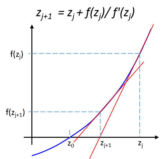
Figure 1. Schematics of the Newton solution method, where z represents the vector of solution variables and f(z) represents the solution function.
Several options of the Coupled command can be used explicitly to determine:
- The maximum number of iterations allowed:
Coupled (Iterations=15){ <set of equations> } - The precision of the solution:
Coupled (Digits=4){ <set of equations> } - The linear solver that must be used:
Coupled (Method=ParDiSo){ <set of equations> } - Whether the solution is allowed to be damped over a number of iterations:
Coupled (LineSearchDamping=0.01){ <set of equations> }
For more details about the Newton solver controls, see Section 9.3.2 Nonlinear Solver Controls.
6.2 Achieving a Good Initial Guess
For the Newton scheme, it is crucial to have a good initial guess. Without a good initial solution, your subsequent Quasistationary or Transient sweep might fail from the beginning.
For most applications, it is best to start by first solving the Poisson equation alone, followed by the Coupled statement, which solves the transport equations all together self-consistently:
Solve {
  Poisson
  Coupled { Poisson Electron Hole }
  ...
}
There are situations where solving the initial Poisson equation might require more iterations and also solution damping. You might need to apply extra options if the density gradient or trap models are activated. To ensure that the initial solution converges, specify LineSearchDamping and also allow for a large number of iterations.
The value assigned to LineSearchDamping determines the factor by which updates applied to the solution variables can be damped. The factor varies between 0 and 1. By default, no damping is performed (LineSearchDamping=1). The smaller the LineSearchDamping value, the smoother the convergence obtained, but more iterations are required to obtain the solution. Therefore, you should typically use it with an increased value for Iterations:
Solve {
  Coupled(
    LineSearchDamping= 1e-4
    Iterations= 100
  ) { Poisson eQuantumPotential }
  Coupled { Poisson Electron Hole }
  ...
}
In some (rare) cases where converging the initial guess is difficult to achieve, requesting extra Gummel iterations for the system of equations with the larger relative error (a smaller value of Digits) helps to converge the entire system of equations. To activate the Gummel iterations, use the Plugin command. For example:
Solve {
  Coupled(
    Iterations= 100
    LineSearchDamping= 1e-4
  ) { Poisson eQuantumPotential }

  Plugin(Iterations=10 Digits=3) { Poisson Electron Hole }

  Coupled { Poisson Electron Hole }
  ...
}
6.3 Optimizing the Nonlinear Solver Performance
While running Quasistationary or Transient device simulations, the keyword Iterations sets the maximum number of Newton iterations per step (20 by default). Due to the Newton method quadratic convergence, usually 3–6 iterations are sufficient to obtain the next solution. If a solution is not found after 15–20 iterations, it becomes increasingly unlikely that a solution will be found for a given step size. Therefore, it is often faster to limit the number of iterations, and to let the current Newton step fail, and restart it with a smaller time step, as shown in Figure 2.
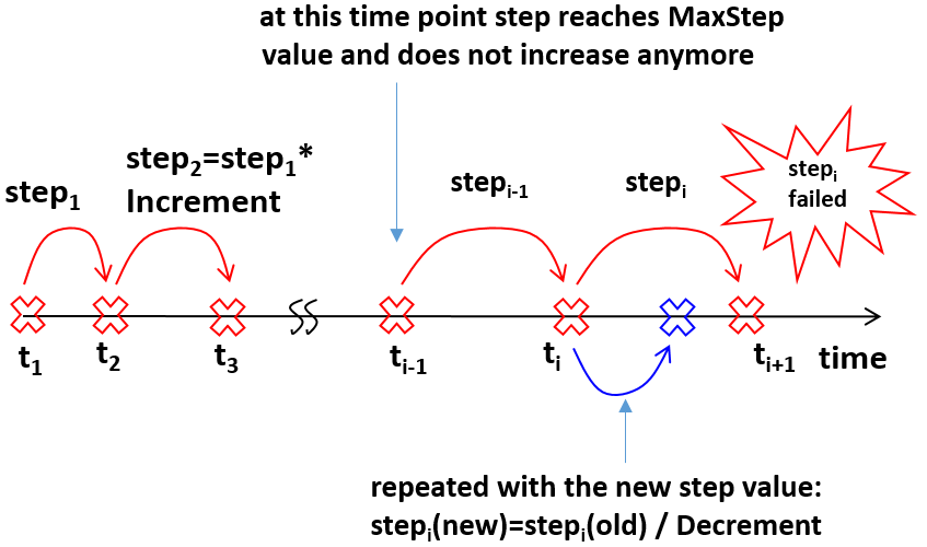
Figure 2. Schematics of the time-step incremental strategy. (Click image for full-size view.)
Two scaling factors are used for this – Increment and Decrement. For Transient simulations, Increment and Decrement values are used exactly as specified in the Transient section:
Transient (
  InitialTime=0 FinalTime=100e-11
  InitialStep=1e-11 Increment= 1.4 Decrement= 2
  MaxStep=5e-11 MinStep=1e-15
){ Coupled{ Poisson Electron Hole } }
For steady-state simulations, the Increment value also depends on the number of iterations in a previous step, according to the following formula:
\[ \text"Increment"(t_{i}) = 1 + \text"max"(0,(\text"Increment" - 1) (1 - {x}/{0.75})) \html" ," \] \[ x= {\text"iterations"(\text"step"_{i-1}) -1} / {\text"Iterations"} \]
By default, the same value (2) is used for both Increment and Decrement. It is recommended to apply a smaller value for Increment than used for Decrement to avoid back and forth time-step jumping in the case of nonconvergence.
For more details about the Newton solver controls for 3D device simulations, see Section 9.3.2 Nonlinear Solver Controls.
For transient simulations, you can use abrupt piecewise linear voltage or current drives. To resolve the steep gradients of the input signal, you can use the TurningPoints statement as a parameter in the Transient section, which instructs the solver about the maximum time steps to be used at specific time points or within specific intervals of time. An example of using TurningPoints is contained in the command file sdevice1_des.cmd of the Sentaurus Workbench project Applications_Library/GettingStarted/sdevice/CMOSInverter discussed in Section 3.3 Transient Sweep.
6.4 Using the Extrapolate Option
By default, at each bias step for a Quasistationary sweep or at each time step for a Transient sweep, the initial guess for the next Newton iterations is taken as the solution from the previous step.
For Quasistationary sweeps, you must always use the Extrapolate option:
Math { ...
  Extrapolate
}
In this case, the initial guess for the next Newton iterations is taken as a linear extrapolation from the last two solutions (see Figure 3). Usually, this option significantly improves convergence, which also helps Sentaurus Device to make larger bias steps.
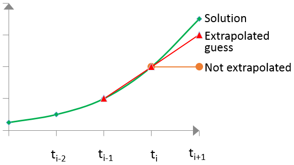
Figure 3. Schematics of the solution extrapolation method.
In some situations such as fast transient ramps, activating extrapolation can lead to convergence difficulties. In such cases, you can give second order extrapolation a try Extrapolate(Order=2)
Quasistationary (
  Goal { ... }
  Extrapolate(Order=2)
) { Coupled {Poisson Electron Hole} }
By default, Sentaurus Device uses extrapolation for all equations from a Coupled command, but you can exclude some equations from this list by specifying equations to be excluded as parameters of the Exclude option:
Quasistationary (
  Goal { ... }
  Extrapolate(Exclude(Poisson Hole))
) { Coupled { Poisson Electron Hole } }
If Extrapolate is switched on globally in the Math section, then you can switch it off locally inside a corresponding Quasistationary or Transient command using -Extrapolate:
Transient ( ...
  -Extrapolate
) { Coupled { Poisson Electron Hole } }
6.5 Determining the Convergence of the Newton Solver
When you run Quasistationary or Transient tasks with the Newton method, the solver convergence is checked against two criteria:
- Global error criterion: \(\text"error"\; = 1/ε_R 1/N ∑↙{e,i}{|z(e,i,j)-z(e,i,j-1)|} / {|z(e,i,j)|+z_{\text"ref"}(e)} < 1\)
- RHS norm criterion: \(\text"RHS"\; = ||A ⋅ x - b|| <\) RHSmin
The Newton solver quits the iterations if either criterion is met. Here, \(z\) indicates the corresponding solution variable, \(e\) refers to the equation, \(i\) denotes the node number, \(j\) corresponds to the iteration, and \(N\) corresponds to the total number of unknowns (number of nodes multiplied by the number of solution variables). The relative error \(ε_R\) corresponds to 10-Digits. The reference error parameter \(z_{\text"ref"}(e)\) can be set through ErrRef(<equation>).
For a well-converging Newton step, you can see in the log file that the error decreases (quadratically) and the RHS also reduces from iteration to iteration:
Iteration   |Rhs|      factor     |step|     error   #inner  #iterative  time
------------------------------------------------------------------------------
    0      2.93e+04                                                      0.54
    1      1.43e+06   1.00e+00   8.91e-02   1.25e+03    0         1      3.22
    2      2.46e+00   1.00e+00   1.30e-02   4.95e+02    0         1      5.96
    3      1.38e-02   1.00e+00   1.37e-03   5.65e+01    0         1      8.73
    4      1.01e-05   1.00e+00   2.57e-05   8.21e-01    0         1     11.43
Finished, because...
Error smaller than 1 ( 0.820967 ).
For a nonconverging Newton step, the error and the "right hand side" no longer decrease and fluctuate:
Iteration   |Rhs|      factor     |step|     error   #inner  #iterative  time
------------------------------------------------------------------------------
    0      2.69e+03                                                     0.61
    1      4.99e+06   1.00e+00   2.09e-01   3.81e+03    0         1     4.82
    2      6.34e+02   1.00e+00   2.55e-01   2.51e+03    0         1     9.13
...
   14      2.05e+01   1.00e+00   3.83e-02   2.12e+03    0         1     59.43
   15      2.84e+01   1.00e+00   1.40e-02   3.31e+02    0         1     63.52
Finished, because...
#iterations larger than 15.
In addition to |RHS| and error, other different quantities are reported, including:
- factor: Represents the damping factor used by the solver. It can be less than 1 if either line search damping or Bank–Rose damping is active.
- |step|: Represents the norm of the update vector.
- #inner: Represents the number of iterations in the damping.
- #iterative: Prints the number of iterations for the ILS solver. In the case of direct solver usage, it either prints 1 or the number of right-hand sides, if multiple right-hand sides are solved simultaneously.
Often, tightening up the Newton error controls helps to converge the simulation. The most relevant parameters here are Digits and ErrRef. In addition, running a simulation in ExtendedPrecision mode helps to resolve such solution fluctuations, which increases the chances of the simulation converging:
Math{ ...
  Digits= 5
  ErrRef(Electron) = 1e8
  ErrRef(Hole)     = 1e8
  ExtendedPrecision
}
For more details about the convergence of the Newton solver in the case of 3D device simulations, see Section 9.3.2 Nonlinear Solver Controls.
6.6 Improving Convergence in Low-Density or Low-Current Regions
This section describes how to improve convergence in low-density or low-current regions.
6.6.1 High-Field Saturation and Avalanche Generation
If the gradient of the quasi-Fermi level rapidly changes but the density does not, convergence can be unstable in regions with small densities. This can be circumvented by introducing a correction density \(n_{0}\) in the equation for the quasi-Fermi potential:
\[ Φ↖{~}_{n} = φ - φ_{\text"ref"} + {χ}/{q} - {kT}/{q} log({n_{0} +n}/{N_{C}}) \]
\[ ∇Φ↖{~}_{n} = ∇φ + {∇χ}/{q} - {k∇T}/{q} log({n_{0} +n}/{N_{C}}) - {kT}/{q} {∇n}/{n_{0}+n} +{kT}/{q}{∇N_{C}}/{N_{C}} \]
The nonzero \(n_{0}\) value stabilizes convergence within regions with small densities but large \(∇Φ\) values. In this case, smoothing is applied to both models that use gradQuasiFermi as a driving force: high-field saturation and avalanche generation. The corresponding reference smoothing densities are provided in the Math section as shown here:
Math {
  RefDens_eGradQuasiFermi_ElectricField= 1e8
  RefDens_hGradQuasiFermi_ElectricField= 1e8
}
These commands activate the smoothing of the driving forces for both the high-field saturation and avalanche generation models. To activate driving force smoothing exclusively for the high-field saturation model, use the following commands:
Math {
  RefDens_eGradQuasiFermi_ElectricField_HFS= 1e8
  RefDens_hGradQuasiFermi_ElectricField_HFS= 1e8
}
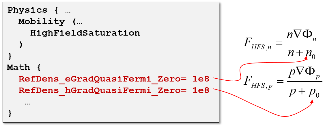
Alternatively, you can use another smoothing option that activates the interpolation between the gradient of the quasi-Fermi potential and the electric field parallel to the interface, which is applied to the driving force of the high-field saturation model:
\[ F_{\text"HFS",n} = {n}/{n+n_{0}} |∇Φ_{n}|\; +\; {n_{0}}/{n+n_{0}} |(I - n↖{\^} \: n↖{\^}^{T})F↖{→}| \]
where \(n↖{\^}\) is a unit vector pointing to the closest semiconductor–insulator interface. To activate this alternative smoothing option, specify the following commands:
Math {
  RefDens_eGradQuasiFermi_EParallelToInterface= 1e8
  RefDens_hGradQuasiFermi_EParallelToInterface= 1e8
}
If you notice that a convergence issue seems to be related to the electron or hole equations, specifically in areas of low carrier densities, then you can consider the RefDens_eGradQuasiFermi_Zero and RefDens_hGradQuasiFermi_Zero parameters, which will effectively damp the driving force of the high-field saturation model within the regions with strong generation–recombination and a low carrier density:
Driving force smoothing is preferred over driving force damping. Try to use it first to circumvent any device simulation convergence issues.
See Section 11.10 Driving Force for Avalanche Generation and High-Field Saturation Models for more details about available model driving forces and drivng force interpolation controls.
6.6.2 Hydrodynamic Transport
If you encounter unrealistically high carrier temperatures in regions with a low-carrier density, then consider limiting the energy relaxation time as a function of the carrier density with:
Math { ...
  RelTermMinDensity= 1e4
  RelTermMinDensityZero= 1e8
}
6.7 Debugging Newton Solver–Related Convergence Issues
This section provides information about how to debug convergence issues related to the Newton solver.
6.7.1 CNormPrint
To have a sense of which equation might be causing poor convergence, activate the printing of the largest error for each equation after each Newton iteration with CNormPrint:
Math { ...
  CNormPrint
}
You will find the information about the vertex where the largest error occurs, its coordinates, and the value of the solution variable being printed after each Newton iteration. For example:
Iteration   |Rhs|      factor     |step|     error   #inner  #iterative  time
------------------------------------------------------------------------------
    0      2.91e+08                                                      0.77
C-norm_equation  max_error vertex      coordinate [um]      value
 poisson:      3.688e-03 5303  (1.831e-02, -1.390e-02) -7.705e-04
 eQuantumPot:  1.595e-03 5380  (1.831e-02, -3.824e-02) -9.692e-03
 electron:     1.152e-02 5512  (1.464e-02, -2.433e-02)  2.478e+15
 hole:         2.710e-03 1665  (2.197e-02,  0.000e+00)  5.720e+11
 eTemperature: 1.808e-03 5295  (2.380e-02, -3.128e-02)  1.242e+03
 lTemperature: 3.684e-05 1776  (2.288e-03,  4.867e-02)  3.181e+02
...
To identify a problem, look at this output only when the Newton steps start to fail. Look for entries where the max_error is of the order of 1 or larger. This shows for which equation the solver is struggling. In addition, if you see that a large error occurs repeatedly at the same vertex or in the same area (see coordinate), look carefully at the mesh in that area; it might be inappropriate.
6.7.2 NewtonPlot
Sentaurus Device can write the spatial values of solution variables, errors, the RHS, and the solution updates to a so-called NewtonPlot file. The NewtonPlot files then can be read into Sentaurus Visual for examination.
Sentaurus Device writes information to a NewtonPlot file during execution of a Quasistationary or Transient command when the step size decreases below a certain value. Use the NewtonPlot keyword in the File section to specify a file root name for the generated plots. This name can contain up to two C-style integer format specifiers (for example, %d). If present, for the file name generation, the first one is replaced by the iteration number in the current Newton step and the second is replaced by the number of Newton steps in the simulation:
File {
  ...
  NewtonPlot= "n@node@_NP_%d_%d_des.tdr"
}
Specify the NewtonPlot statement in the Math section to explicitly activate file-writing:
Math {
  ...
  NewtonPlot(<options>)
}
Refer to the Sentaurus™ Device User Guide for the corresponding set of NewtonPlot options.
Figure 4 shows an example of what can be plotted after the NewtonPlot command is executed. You can see the distribution of the relative error of the hole density inside the device and other datasets that can be plotted.
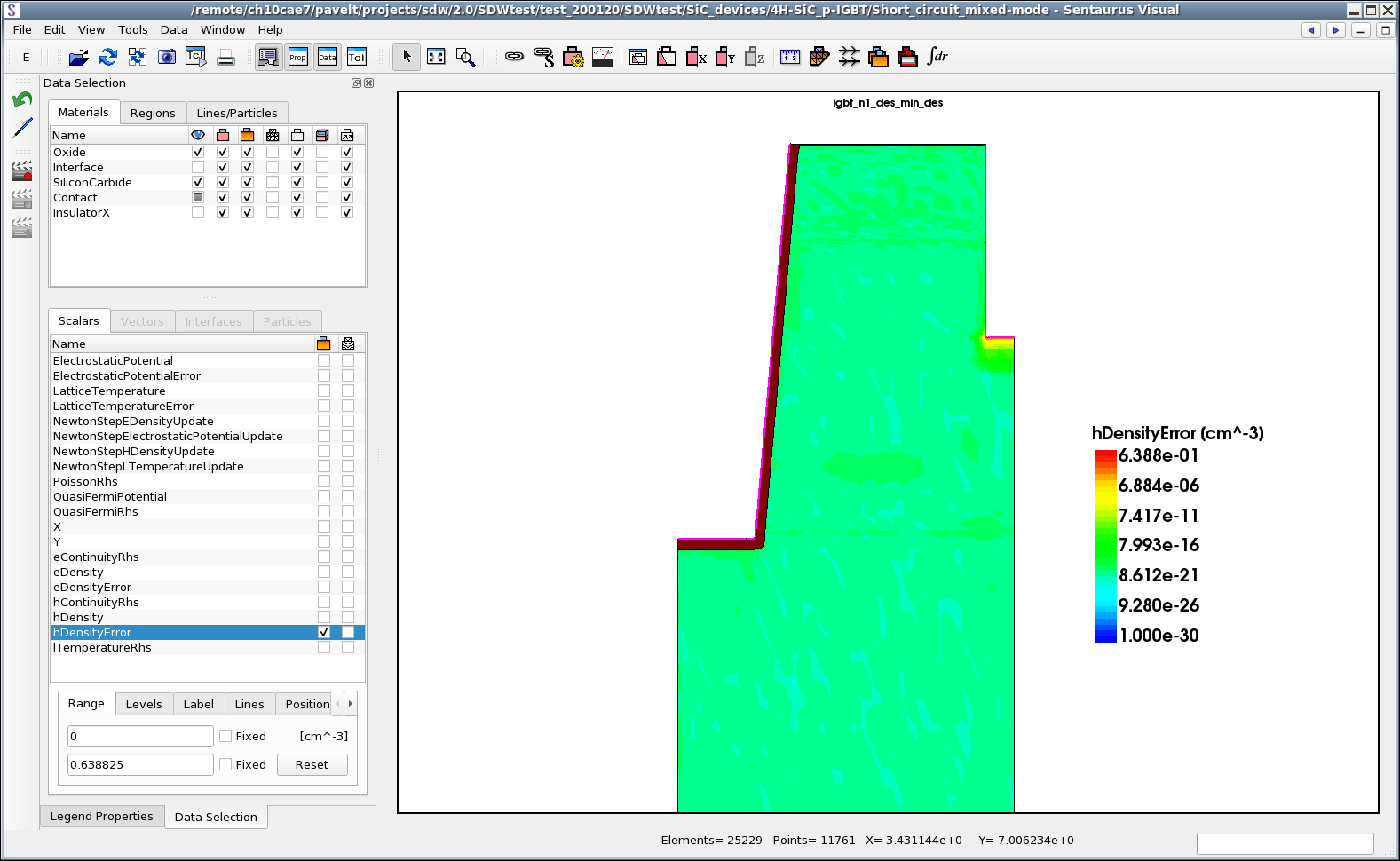
Figure 4. Typical visualization in Sentaurus Visual of dataset after NewtonPlot command is executed. (Click image for full-size view.)
6.7.3 AutoCNPMinStepFactor and AutoNPMinStepFactor
In the case of nonconvergence, Sentaurus Device automatically activates the CNormPrint and NewtonPlot commands, if the following criteria are met:
- For CNormPrint: step size < AutoCNPMinStepFactor * MinStep
- For NewtonPlot: step size < AutoNPMinStepFactor * MinStep
By default, this will print additional information about the last successful Newton iteration and also will generate a *_des_min.tdr file for further debugging. The AutoCNPMinStepFactor and AutoNPMinStepFactor values can be specified in the Math section of the command file:
Math {
  AutoCNPMinStepFactor = <float> #default = 2.0
  AutoNPMinStepFactor  = <float> #default = 2.0
}
For 3D device simulations, such files can use significant disk space. To deactivate file-writing, assign zero values to the corresponding step factor.
Copyright © 2022 Synopsys, Inc. All rights reserved.