 main menu
| module menu
| << previous section
| next section >>
main menu
| module menu
| << previous section
| next section >>
Sentaurus Device Electromagnetic Wave Solver
5. Special Focus: Using CODE V Excitation
5.1 Overview
5.2 Preparing EMW for CODE V Excitation
5.3 Extracting Excitation Fields From CODE V
5.4 Using CODE V Excitation Fields in EMW
Objectives
- To learn how to extract excitation fields suitable for EMW from the Synopsys CODE V® tool.
- To understand how to import CODE V excitation fields into EMW.
5.1 Overview
The beam synthesis propagation (BSP) method of CODE V is often useful within optical systems where beam divergence due to diffraction can be significant, for example, camera lenses for image sensors. EMW offers an interface to BSP to import optical fields on 2D cross sections of CODE V and to use them as excitation.
As CODE V does not support the export of H-fields, complex E-fields must be exported at two different planes, from which EMW then can reconstruct the H-field. However, for the reconstruction of the H-field to be precise enough, interpolation must be avoided. Therefore, the distance of the export planes in CODE V must correspond to the grid spacing at the excitation plane of the EMW grid.
To import a CODE V excitation into EMW, you must:
- Set up the EMW simulation and determine the grid spacing at the excitation plane.
- Define 2D cross-sectional slices in CODE V using adequate grid spacing and width, and export the fields.
- Run the EMW simulation using CODE V excitation.
The following sections describe these steps in detail using a standard camera lens from CODE V and a planar air–silicon interface for EMW.
The complete CODE V project is available as codev-excitation.zip.
The complete EMW project can be investigated from within Sentaurus Workbench in the directory Applications_Library/GettingStarted/emw/import-codev.
5.2 Preparing EMW for CODE V Excitation
Before exporting the excitation field in CODE V, you need to know the exact grid spacing and width of your excitation plane. Usually, this can be extracted directly from within Sentaurus Visual. However, if the tensor mesh is too big, it is faster to run a test EMW simulation with a few time steps, to create a 2D plot, and to extract the coordinates in Sentaurus Visual from the 2D plot.
An example of how to set up a 2D plot can be found in the project Applications_Library/GettingStarted/emw/simple3d in the emw_eml.cmd command file.
In this example, you can open the tensor mesh n3_msh.tdr directly in Sentaurus Visual and use the probe tool to find the excitation planes located at z1 = -0.3125 and z2 = -0.25.
During probing in Sentaurus Visual, hold the Ctrl key to have the probe tool snap to the vertex and to give you the exact coordinates.
5.3 Extracting Excitation Fields From CODE V
To run the CODE V part:
- Download the CODE V project files as codev-excitation.zip.
- Unzip the archive to the CODE V user directory typically: c:\CODEV\CVUSER.
- Edit the following lines in emw-export.seq.txt
to match your EMW simulation:
^gridWidth == 1e-3      ! Width of EMW grid in [mm]
^npts      == 60        ! Number of exported grid points, look at snmesh log.
^planeZ1   == -3.125e-3 ! z coordinate of 1st excitation mesh plane in [mm]
^planeZ2   == -2.5e-3   ! z coordinate of 2nd excitation mesh plane in [mm]
- Open CODE V.
- In the Command Window, type: tow in emw-export
- Copy the excitation fields data_z1.dat and data_z2.dat to your Sentaurus Workbench project.
As the exported CODE V fields must match your EMW grid spacing, you must rerun CODE V whenever you change the EMW grid.
5.4 Using CODE V Excitation Fields in EMW
To use the CODE V fields as excitation in EMW, a CodeVExcitation section must be defined in the emw_eml.cmd file:
CodeVExcitation {
   InputDataFile    = {"@pwd@/data_z1.dat", "@pwd@/data_z2.dat"}
   AnchorPoint1     = {-0.5, -0.5, -0.3125}
   AnchorPoint2     = {-0.5, -0.5, -0.25}
   Wavelength       = 550
   Nrise            = 5
}
Therein, the InputDataFile defines the input file names.
AnchorPoint1 and AnchorPoint2 set the reference point of the smallest x,y coordinates of the CODE V field data and the z-coordinate of the excitation planes. The propagating E-field is assumed to flow in the direction from z1 to z2, so in this example in the +z-direction.
Other keywords such as Wavelength and Nrise have their usual meaning (see Section 2.6 PlaneWaveExcitation Section).
In addition, the keyword AmplitudeScaling can be used to scale the imported excitation field.
Figure 1 shows the resulting optical generation in silicon; half of the structure is blank to see the depth profile. Clearly, the circular focused beam spot is visible, and the depth profile shows a convergent beam into the silicon.
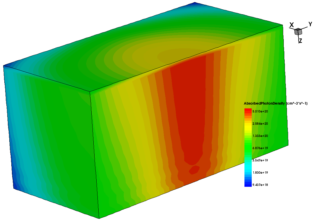
Figure 1. Optical generation in silicon. (Click image for full-size view.)
CODE V excitation has the following restrictions:
1. The incident light propagation is limited to the z-direction.
2. Only the following boundary conditions are allowed:
– CPML at all sides.
– periodic at the X- and Y-sides, and CPML at the Z-side.
3. Only 3D simulations are supported.
4. The excitation plane must be in vacuum (that is, n=1, k=0).
main menu | module menu | << previous section | next section >>
Copyright © 2022 Synopsys, Inc. All rights reserved.