
Sentaurus Device Electromagnetic Wave Solver
4. Best Practices for Image Sensor Simulations
4.1 Overview
4.2 Structure Generation
4.3 Meshing
4.4 EMW Simulation
4.5 Result Extraction
Objectives
- To learn how to most efficiently set up, run, and evaluate image sensor simulations with EMW.
4.1 Overview
An EMW simulation project consists of several components including structure generation, mesh generation, optical simulation, and evaluation of results. For a successful and efficient simulation, the smooth interplay of these components is crucial. Figure 1 shows the tool flow of a simple EMW project containing all the important components.
- pixel
- The electrical device generation, here performed in Sentaurus Structure Editor, but could also be accomplished in one or several Sentaurus Process steps.
- beol
- Additional optical components usually present in the back-end-of-line (BEOL) and typically not required for electrical simulation; typically performed in Sentaurus Structure Editor.
- emw
- Performs the optical simulation itself.
- svisual
- Sentaurus Visual tool for evaluating results such as absorption in regions and photon fluxes.
- movie
- Sentaurus Visual tool to compile a movie in GIF format from a time series of snapshots.
The complete project can be investigated from within Sentaurus Workbench in the directory Applications_Library/GettingStarted/emw/simple-cis.

Figure 1. Sentaurus Workbench Project. (Click image for full-size view.)
4.2 Structure Generation
CMOS image sensor (CIS) simulation setups can be very complex and usually have many input parameters such as pixel size, substrate thickness, and wavelength.
The following sections introduce a few concepts to illustrate how complex setups can be broken down and organized in a way to allow for a more efficient workflow.
4.2.1 Global Parameters
For an efficient setup, it is helpful to define input variables in one place as global parameters, so they can be set in a single place and referred to in different tools consistently. For this purpose, the first tool pixel has an additional file pixel_var.txt that is loaded in the command file of the first tool with:
#includeext "pixel_var.txt"
and only serves the purpose to define hidden Sentaurus Workbench variables with #seth statements that can be accessed by using the usual @var@ syntax in any subsequent input file. For example, the pixel size and substrate thickness are defined in pixel_var.txt with:
#seth w_pixel 1
...
#seth t_sub 2
In the file pixel_dvs.cmd, these parameters are then accessed to create the silicon substrate as follows:
(sdegeo:create-cuboid
  (position 0 0 0)
  (position @w_pixel@ @w_pixel@ (- @t_sub@))
If you looked at the created boundary file (by selecting the node and clicking the Quick Visualize toolbar button), you might have noticed that the substrate thickness is actually 1 μm and not 2 μm as defined in pixel_var.txt. This is due to the fact that @t_sub@ has been redefined as a Sentaurus Workbench parameter in the Sentaurus Workbench table; Sentaurus Workbench parameters in the table always overwrite any #seth definition. This behavior allows you to easily introduce variations of a certain #seth variable; you simply create a corresponding Sentaurus Workbench parameter in the table.
In addition to global parameters, there are extracted parameters that can be used in subsequent tools. This is accomplished by writing variable–value pairs into the output file of the tool. For example, in the pixel tool, the minimum z-coordinate of the device is extracted by the following lines:
(define zmin (sde:min-z (get-body-list)))
(sde:ft_scalar "zmin " zmin)
This outputs a line like the following to the corresponding n3_dvs.out file:
DOE: zmin -1
To label @zmin@ as a hidden parameter, so it does not appear in the results table of Sentaurus Workbench, you add a corresponding #seth definition at the beginning of pixel_dvs.cmd:
#seth zmin x
To see a list of available @-parameters and variables at a certain node, you can always select that node, and then right-click the node and choose Node Explorer (or press the F7 key), then go to the Node Data tab (see Figure 2).
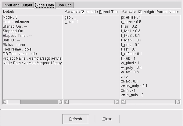
Figure 2. Node Explorer showing available parameters. (Click image for full-size view.)
When using extracted variables in subsequent tools, for example, @zmin@ from the tool pixel is used in the EMW command file, you must ensure that, during preprocessing, a reasonable value already exists for it. Otherwise, preprocessing of the EMW command file will fail. This can be achieved by checking the value of @zmin@ at the beginning of the emw_eml.cmd file and stopping preprocessing if it is not adequate:
#if @<![string is double t_Me1 ]||![string is double zmin ]||![string is
double zmax_Me1 ]>@
EMW requires numeric values for extraction variables during preprocessing.
Run Sentaurus Structure Editor nodes first.
#exit
#endif
4.2.2 Organizing Structure Editor Input Using Splits
Optical structure generation typically results in lengthy scripts. To maintain a good overview, it is advisable to break up the script into splits using the preprocessor construct:
#header
initialization part
#endheader
initial commands

#split @A@
commands of split A

#split @B@
commands of split B
To make the split work, the Sentaurus Workbench parameters @A@ and @B@ must be defined for the tool. This will execute for the first node of the tool:
initialization part
initial commands
for the node under @A@:
initialization part
commands of split A
and for the node under @B@:
initialization part
commands of split B
Sentaurus Workbench ensures that, at the end of a split, the results are saved and, at the beginning of the next split, they are reloaded.
Looking at Figure 1, you will notice that the tool beol has three yellow nodes. This is due to the splits introduced in beol_dvs.cmd as follows:
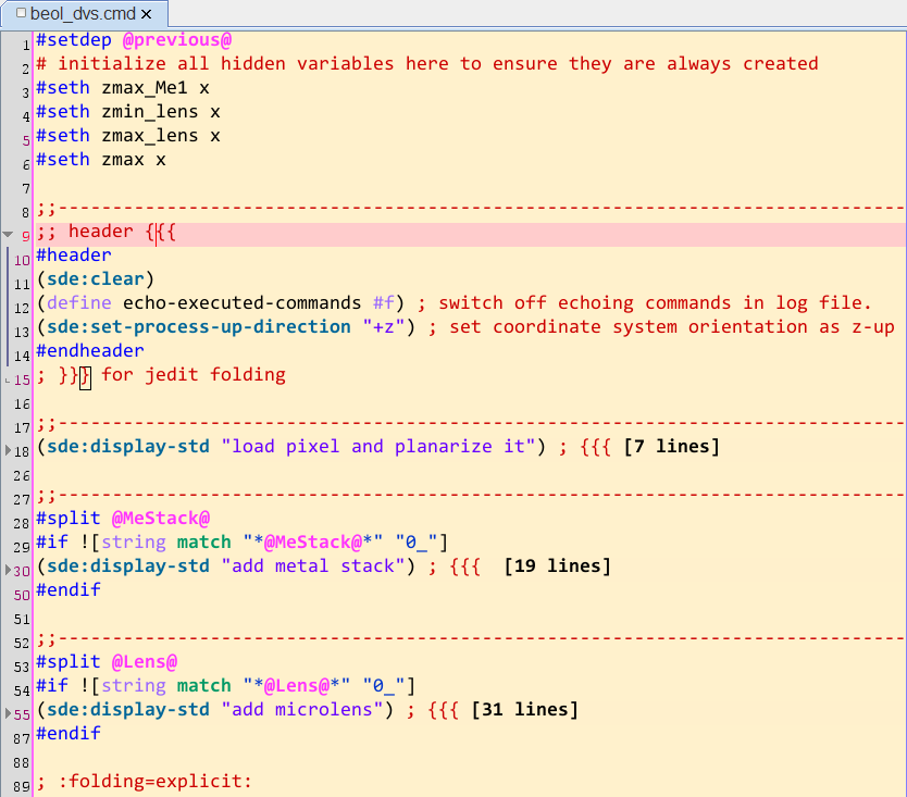
Figure 3. jEdit demonstrating splits and explicit folding. (Click image for full-size view.)
The first initial node of the beol tool loads the pixel from the previous step and planarizes it by filling voids with Oxide. The second node under @MeStack@ adds the metal stack, and the final node under @r_Lens@ adds the microlens.
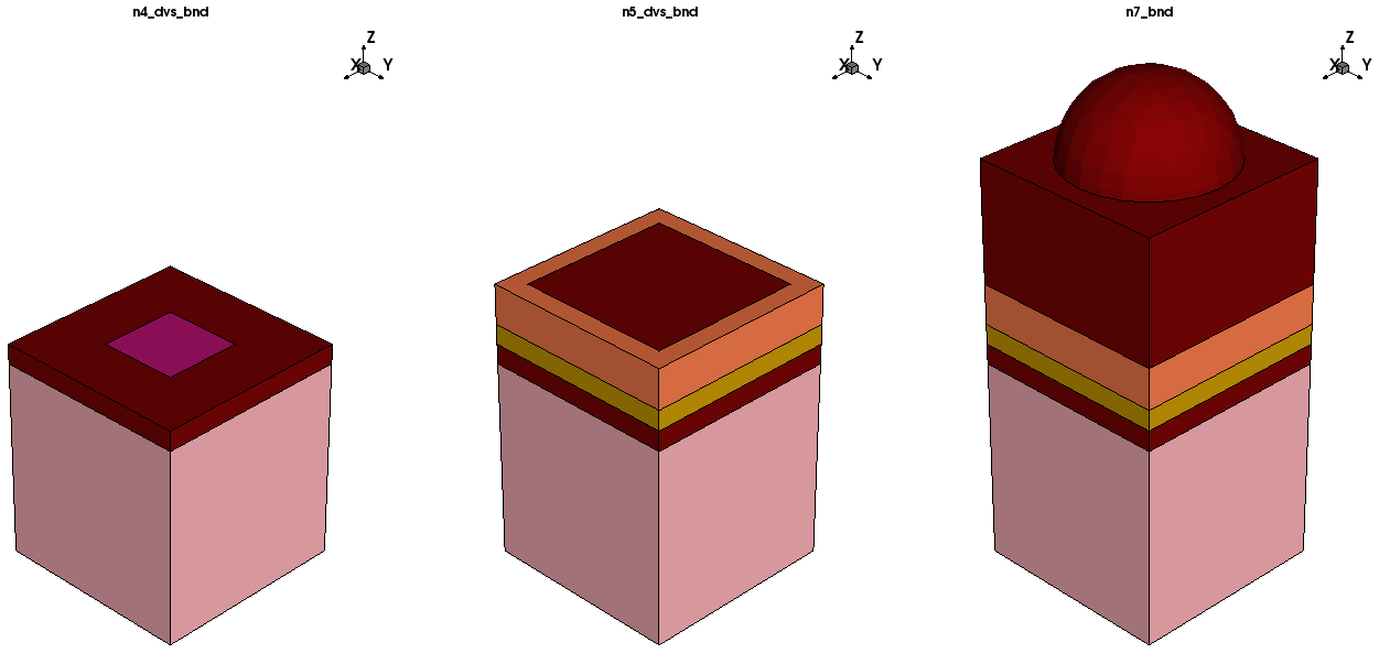
Figure 4. Resulting structure of the three splits. (Click image for full-size view.)
4.2.3 Maintaining Overview With Folding in jEdit
Looking again at Figure 3, you can see how explicit folding in jEdit helps you to maintain the overview in long scripts. Everything between {{{ and }}} can be collapsed and expanded using the Folding menu. Folds are marked by a small triangle close to the line numbers and the number of collapsed lines is appended. To activate explicit folding, add the line ; :folding=explicit: to your file.
4.3 Meshing
For the basic principles of how to create a tensor mesh, see the Sentaurus Mesh module, Section 7. Using the Tensor-Product Mesh Generator.
4.3.1 Courant Criteria
CIS devices are usually complex and are often generated with the help of masks, which easily leads to tiny misalignments of boundaries across the structure. These small misalignments then propagate further into very small tensor cell sizes and can impact the maximal stable time step defined by the Courant criteria:
$Δt_{stable} = 1 / {c/n √{1/{Δx}^2+1/{Δy}^2+1/{Δz}^2}}$
which, in one dimension, reduces to the following equation:
$Δt_{stable,1d} = {n Δx} / {c}$
Therefore, the stable time step is limited by the smallest edge length. Note that the cells in the region with lowest n – most often gas around the lens – are the most critical for the overall time-step computation.
So it is crucial to avoid very small cell sizes in general, but understanding which region is actually limiting the stable time step is a more complex task. Sentaurus Mesh can help you here: setting verbosity=3 in the IOControls section (see snmesh_msh.cmd) prints the stable time step for each material at the end of its log file (n12_msh.log):
Summary:
--------
Copper:  tcourant=n/a minCellSize=(0.01, 0.01, 0.01) cells=72000
Gas:     tcourant=2.223761e-17s minCellSize=(0.01, 0.01, 0.02) cells=204419
Nitride: tcourant=4.279048e-17s minCellSize=(0.01, 0.01, 0.014286) cells=70000
Oxide:   tcourant=2.444004e-17s minCellSize=(0.01, 0.01, 0.007143) cells=611181
PolySi:  tcourant=6.545171e-17s minCellSize=(0.01, 0.01, 0.007143) cells=22400
Silicon: tcourant=6.791883e-17s minCellSize=(0.01, 0.01, 0.007576) cells=1320000
--------
global:  tcourant=2.223761e-17s minCellSize=(0.01, 0.01, 0.007143) cells=2300000
This summary tells you that the stable time step will be 2.223761e-17 s (last line), and it is limited by the Gas region. In addition, you can see that relaxing the mesh in the Gas does not increase the stable time step much, as the next limiting region, the Oxide region, has a slightly higher stable time step. Therefore, the Oxide would have to be coarsened as well to achieve a significantly larger time step.
Dispersive regions, like Copper, do not contribute to the stable time-step computation.
4.3.2 NPW and maxNPW Refinement
In general, for CIS devices, it is convenient to use the nodes per wavelength (NPW) refinement. However, similar to the general pairwise definition of refinements in a minimum and maximum notation, NPW also allows for defining a maximum NPW using the command maxNPW. Usually, the NPW settings are controlled by Sentaurus Workbench parameters for all directions @NPW@ plus a separate one in each propagation direction @NPWz@.
It is common practice to increase the NPW value by 1.5x in the propagation direction to achieve more accurate results. A convenient way to control all of the maximum NPW values accordingly is to define one parameter @fmax@ and then multiply all NPW parameters by it as @<NPW*fmax>@. The typical @fmax@ is in the range of 1..2. This results in the following typical mesh command file:
    NPWx = @npw@
    NPWy = @npw@
    NPWz = @npwz@
    maxNPWx = @<fmax*npw>@
    maxNPWy = @<fmax*npw>@
    maxNPWz = @<fmax*npwz>@
Click to view the primary file snmesh_msh.cmd.
4.4 EMW Simulation
This section describes how to set up EMW efficiently so it fulfills the different requirements during project development, from fast running at the beginning to optimized turnaround time for variations.
Click to view the primary file emw_eml.cmd.
4.4.1 Controlling Termination of the Simulation
One of the main simulation settings of EMW is the break criteria or tolerance usually introduced as the Sentaurus Workbench parameter @tol@. However, depending on what you simulate, there might be better choices to terminate the simulation. In this setup, depending on the range of @tol@, different break criteria are applied:
- Tolerance [0 < @tol@ < 1]
- The simulation ends if the maximum deviation of the E-fields compared to the
previous check is less than @tol@.
+ Automatic convergence detection.
- Increases turnaround time, especially on GPU.
- @tol@ should not be confused with the simulation error. It is an empirical number that must be adapted for each application and can depend on wavelength or incident angle or both; typical values are 1e-3...1e-5. - TotalTimeStep [@tol@=0, or 1000 ≤ @tol@]
- The simulation ends after @tol@ number of time steps.
+ Very fast, as no detector is required.
+ Use TotalTimeStep = 1 to quickly produce cuts to check setup, structure, and meshing.
- You need to know when simulation will stop.
- Propagation distance might vary: propagation distance = # of timesteps × timestep
- ct [1 ≤ @tol@ < 1000]
- The simulation ends after the light in vacuum would have propagated this
distance d = c × t in μm.
+ Very fast, as no detector is required.
+ Propagation distance is well defined even when time step varies.
+ The value of ct has a descriptive meaning.
- You need to know how far the light must propagate to reach a certain accuracy.
Therefore, in a typical project development, you would first use @tol@ = 0 to visualize the tensor mesh cuts and check whether all regions are resolved in a reasonable manner.
Then, you would run a few @tol@ = 0.1 or @tol@ = 1001 with a very coarse mesh to see whether all the scripts are running through as expected.
Next, you would decrease @tol@ = 1e-3..1e-5 and play with the refinement to find the optimum between turnaround time and accuracy (for example, deviation of R+T+A from 1). The result extraction, in the next section, always returns the propagation distance ct, so you will develop a sense of the value for ct for this particular structure
For a large design-of-experiments (DoE), especially in conjunction with GPU, it is advisable to use @tol@=<ct>, where <ct> is the optimum value as determined in the previous step. This optimizes the turnaround time by deactivating the detector.
4.4.2 General Considerations for Plotting
CIS structures usually have a few million cells to a couple of hundred cells. Therefore, often you cannot save the full 3D structure for visualization in Sentaurus Visual. To solve this issue, you can do one of the following:
- Save only a subset of regions using the Plot keyword region.
- Save your data onto a coarser mixed-element grid.
- Save 2D cuts instead of full 3D.
Option 1 is usually still too large because the silicon domain typically is still too large.
Option 2 can be used especially when a subsequent Sentaurus Device simulation is performed. However, often it is interesting to see interference patterns that otherwise might be lost during interpolation onto a coarse grid.
As a minimum set of plot quantities, the following is a good starting point:
Quantity = {AbsElectricField, CplxRefIndex, CplxExtCoeff}
The magnitude of the electric field AbsElectricField is the most commonly used quantity to investigate optics. The n&k values CplxRefIndex and CplxExtCoeff are always useful to understand the optical device behavior. In addition, if displayed as contour lines, it can be used to mimic region boundaries during visualization (see Figure 5).
Avoid the quantity region. This requires a more complex format for storage in TDR files and comes with a significant performance penalty for writing.
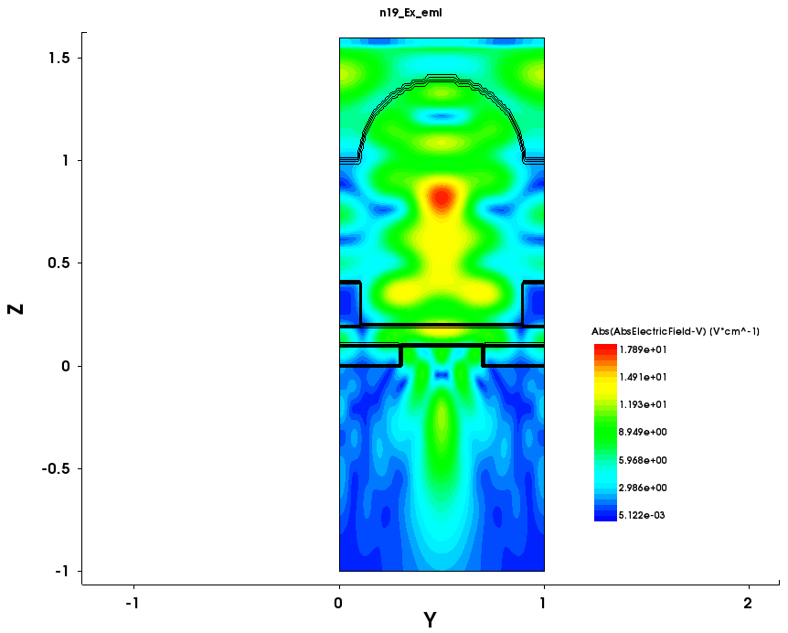
Figure 5. Visualizing the structure using CplxRefIndex as contour lines to indicate region interfaces. (Click image for full-size view.)
In general, it is helpful to turn plotting completely on and off with a single switch, for example, to optimize turnaround time or disk space when running large DoEs or performance optimizations. In this template, this is accomplished by adding plot to the Sentaurus Workbench parameter @model@.
In addition, it is useful to control the transient plotting of snapshots taken during light propagation, for example, to investigate the dynamics of light propagation, which can also be converted to a movie later by using the Sentaurus Visual tool movie. The Sentaurus Workbench parameter @movieCuts@ takes a list of plot section names, for example Ex, which then will be plotted during light propagation. @movieTickStep@ is used to control the number of steps between two subsequent plots.
4.4.3 Working With Cuts
For CIS devices, usually one vertical x-cut and y-cut through the middle of the structure and several horizontal z-cuts are helpful to investigate the optical behavior. While the two vertical cuts are straightforward, real structures might require dozens of z-cuts, each of them requiring a separate Plot section. This repetitive work can be streamlined using Tcl preprocessing. First, you define a list of label and z-cut position pairs:
!(
set plotZcuts [subst {
  "Me1" @<zmax_Me1-t_Me1/2.>@
  "poly" @<(zmax_poly+zmin_poly)/2.>@
  "SiTop" -0.01
  "bot" @zmin@
}]
...
Note how you are using preprocessing variables such as zmax_Me1 extracted by Sentaurus Structure Editor to achieve a self-consistent definition of geometric parameters.
Second, for each entry, you create a corresponding Plot section:
...
foreach {label z} $plotZcuts {
  puts "Plot {"
  puts "  Name = \"n@node@_Ez$label\""
  puts "  Quantity = {AbsElectricField, CplxRefIndex, CplxExtCoeff}"
  puts "  PlaneZ = $z"
  ...
}
)!
The same principle of preprocessing can be used to define z-cuts for extractors and sensors.
When visualizing cuts within Sentaurus Visual, the first thing you notice is that, depending on the cut type, the structure might be upside down or labeled with the wrong axis, as EMW saves all plots regardless of their orientation as xy plots. To correct for this, a custom button has been introduced, which assumes that the plot names of the cuts end in x, y, or z and, depending on this, corrects the orientation and axis labels accordingly (see Figure 6).
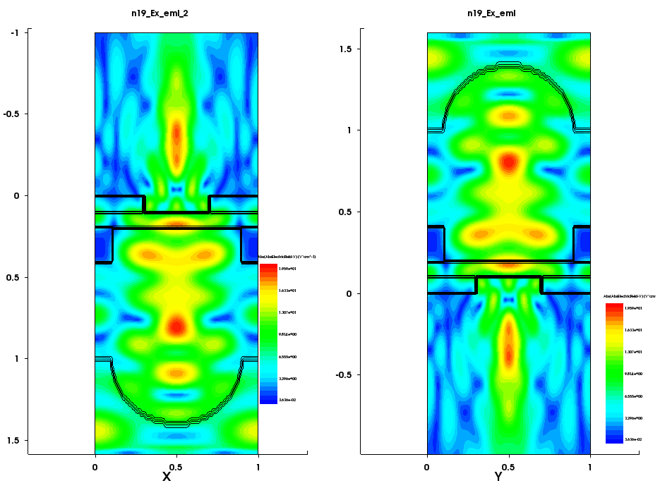
Figure 6. (Left) X-cut as loaded by Sentaurus Visual and (right) after using the custom button with fixed orientation and axis labels. (Click image for full-size view.)
To use this feature, ensure:
- Sentaurus Visual runs in Tcl mode.
- The custom button toolbar is switched on (choose View > Toolbars > CustomButtons). You should see the E of the custom button toolbar for editing it.
- You open Sentaurus Visual from within the simple-cis project.
Then, you should see the fix coordinate system for EMW cuts button in the toolbar as shown in Figure 7.
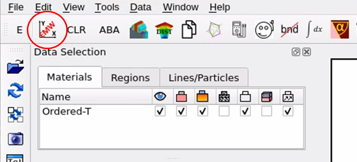
Figure 7. Sentaurus Visual showing custom button to fix axis and orientation of EMW cuts. (Click image for full-size view.)
4.4.4 Using Sensors
Sensors are a very powerful EMW feature to integrate quantities over a volume or surface. Evaluation can occur at the end only or during time propagation, which can provide important insights into how light propagates in the device and also about convergence details. Figure 8 shows the evolution of R,T,A and the deviation of the error |1-RTA|. Obviously, the simulation converged after ct=~60 um as RTA no longer shows significant changes. A smaller error than |1-RTA|=0.005 is not achievable with this mesh.
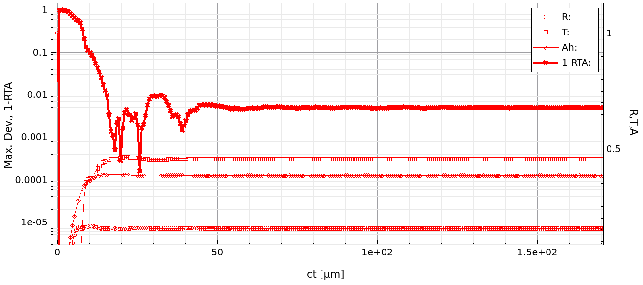
Figure 8. Evolution of R,T,A and 1 – RTA during time given in c · t. (Click image for full-size view.)
As with other extra features, the transient evaluation of sensors requires additional computation time and, therefore, can be switched on by adding transSens to @model@.
It is not advisable to run volume integration sensors for large domains in transient mode, as it can take considerable time.
The most valuable sensors for CIS are reflection, transmission, and absorption sensors (RTA) and region or materialwise volume integration sensors to capture the absorption in specific regions or materials. For RTA, the RTA section of EMW can be used. Which sensors are evaluated can be controlled with the Sensors command.
The log output allows you to set which output quantities are printed to the log file and, consequently, appear as Sentaurus Workbench results. You can choose between R,T,A and the sum of RTA. In addition, the normalized values Rnorm,Tnorm, and Anorm are available with:
$Rnorm = R/(R+T+A)$
Note that the switches for transient evaluation are present in the RTA section as for any sensors, as well. However, when running the sensors in transient, you might want to switch off A in the RTA section, as it is a volume integration over the entire device and might increase runtime considerably.
Due to the staggered grid used in EMW, E- and H-fields must be interpolated to the same location before any further computation such as squaring for the intensity can be performed. To improve accuracy, EMW first squares the E-field and then evaluates the spatial interpolation required by the staggered grid. In this way, interpolation errors are not enhanced by squaring them. This scheme can be used by setting CompatibilityMode=No in the Sensor or RTA section.
Another helpful approach is to use z-cut flux sensors throughout your device, for example, below the lens, or at the top of the silicon, which basically tracks how the flux along the propagation direction in your device varies, thereby giving you a quick insight into where the light "disappears" in your device. The same preprocessing approach as for plots is used to define multiple sensors efficiently:
!(
set dz 0.05 ;# shift in z direction to set flux sensors away from interfaces
set sensorZFlux [subst {
  "lens" [expr @zmin_lens@ - $dz]
  "PolyTop" [expr @zmax_poly@ + $dz]
  "SiTop" 0
}]

foreach {label z} $sensorZFlux {
  puts "Sensor {"
  puts "  Name              = \"F$label\""
  puts "  Quantity          = PhotonFluxDensity"
  puts "  PlaneZ            = $z"
  puts "  Mode              = {Integrate}"
  puts "  CompatibilityMode = No"
  #if [string match -nocase "*transSens*" "@model@"]
  puts "  StartTick         = 0"
  puts "  TickStep          = @movieTickStep@"
  #endif
  puts "}"
}
)!
Note that all sensors shift by a small amount dz to avoid being positioned exactly at an interface.
4.4.5 Troubleshooting Convergence Issues
FDTD simulation can fail for various reasons. This is a list to check for the most common reasons:
- Does the mesh show everywhere at least 5 nodes per wavelength? This is the minimum for a wave to be well-defined in a medium.
- Is the specified tolerance too ambitious? If the reported error in the log tends to stagnate at a certain value, then the chosen mesh might be too coarse to reach the requested tolerance. In this case, relax the tolerance or increase the mesh density.
- Check Nrise. In rare cases, increasing Nrise in the Excitation section up to 30 can help convergence. Nrise sets the number of signal periods before full amplitude of the excitation is reached. A steep function introduces higher order frequencies, which must vanish from the simulation to fulfill steady-state criteria of the harmonic signal.
- Does the simulation include dispersive media? If so, then try to increase Oversampling in the Globals section up to 4. An indication that dispersive media are the problem is when using PEC instead of dispersive media allows the simulation to run successfully. To do so, simply change the DispersiveMedia section to the PEC section, removing the DispersiveMedia-specific options.
4.4.6 Troubleshooting Accuracy Issues
Due to the nature of the staggered grid used in the Yee algorithm commonly used in FDTD, a reasonable judgment of the accuracy can be a real challenge. In general, a finer grid improves accuracy. which is typically measured by the deviation of reflection, transmission, and absorption from 1, so Δε = |1 – R+T+A|.
However, increasing the mesh density not only increases the number of discrete points that must be processed, but also decreases the stable time step to advance the simulation in time according to the Courant criteria (see Section 4.3.1 Courant Criteria). Therefore, more time steps must be calculated for the same propagation distance. So, overall, the feasibility to improve accuracy by increasing the mesh is limited.
Some further considerations before you adjust the global mesh refinement:
- Did the simulation reach stationary state? One indication of this is that, when using a detector, the error values smoothly decrease and eventually drop below the tolerance. For a more detailed picture, run sensors in transient and check the evolution of R, T, A. Increase the simulation time if needed.
- If you see beats in the transient R, T, A signals on a longer time scale, then this might indicate that the excitation signal was ramped up too fast. In this case, increasing Nrise up to 30 will remove higher order modes and result in a smoother evolution of R,T,A (see Figure 9).
- Ensure you have CompatibilityMode=No for your sensors and in the RTA section.
- Try to refine the illuminated interfaces of strong absorbing materials.
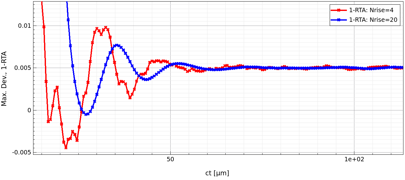
Figure 9. 1 – RTA shows much smoother behavior for larger Nrise. This can be more pronounced for structures showing more optical resonance. (Click image for full-size view.)
4.4.7 Parallelization
EMW offers different parallelization schemes, such as shared-memory parallelization (SMP), distributed processing (DP) using message passing interface (MPI), and hardware acceleration on graphics processing units (GPU).
For CIS, SMP is commonly used in combination with GPU. For very large structures, such as cross-talk simulations, multiple GPUs can be used through MPI.
The number of threads can be controlled in the Globals section by:
Globals {
  NumberOfThreads = @nthreads@
}
where @nthreads@ is a hidden variable defined in emw_eml.cmd, so it can be easily parameterized by introducing a Sentaurus Workbench parameter.
If you own a GPU and you purchased an emw_mpi license, then you can run the time-stepping part of the FDTD simulation on the GPU using the command-line option -hw nvidia, which you can set in the Command-Line Options field of the EMW tool properties. The command-line option -hw none uses CPU only and is the default. In the project, this option is introduced by the Sentaurus Workbench parameter @gpu@. For GPU, it is recommended to use 8 threads. Otherwise, the remaining CPU tasks such as preprocessing (material assignment), detector evaluation, and postprocessing (sensors, extractors) dominate the turnaround time.
4.5 Result Extraction
The major EMW results are shown in the Sentaurus Workbench results table, which originates directly from EMW as well as from the Sentaurus Visual tool svisual. In addition, the Sentaurus Visual tool movie can generate an animated GIF of the light propagation.
4.5.1 Extracted Results
EMW can transfer different quantities such as reflection, transmission, and absorption (R,T,A) directly to the Sentaurus Workbench results table. For details about how to control the output in EMW, see Section 4.4.4 Using Sensors.
However, there are quantities that require more computational effort, such as absorption of certain regions or groups of regions or runtime statistics. These quantities are extracted in the svisual tool run when in batch mode. The command file of this tool is structured into two parts: the first part is executed only in batch mode and the second part is executed only when run in interactive mode described in the next section:
##############################################################################
# B A T C H
if {![info exists runVisualizerNodesTogether]} {
...}
As Sentaurus Workbench respects the order of how result variables appear in the log file, the order of the output can be used to group variables together. First, EMW outputs R,T,A. Second, Sentaurus Visual adds RTA and materialwise absorption, fluxes, propagation quantities, and statistics, grouped into corresponding sections.
| Variable | Unit | Description |
|---|---|---|
| R | 1 | Reflection |
| T | 1 | Transmission |
| A | 1 | Absorption (over entire domain, if @model@ contains noA A=1-R-T) |
| RTA | 1 | R+T+A |
| __ABS__ | __ | Absorption for subdomains, implemented as region or material sensor – no box sensors – whose names start with A |
| ACopper | 1 | Absorption in Copper |
| APolySi | 1 | Absorption in PolySilicon |
| ASilicon | 1 | Absorption in Silicon |
| Asum | 1 | Sum of the absorption of all of the previously mentioned subdomains |
| __FLUX__ | __ | Relative fluxes in propagation direction |
| TF | 1 | Relative flux through the total field sensor TF: 1 for vacuum case, < 1 in case of reflection |
| Flens | 1 | Relative flux at bottom of lens |
| FPolyTop | 1 | Relative flux at top of PolySilicon |
| FSiTop | 1 | Relative flux at top of Silicon |
| __PROP__ | __ | Propagation quantities |
| ct | $μm$ | Total vacuum propagation distance of the simulation |
| Rstep | 1/$μm$ | Number of time steps required per μm vacuum propagation distance |
| __STAT__ | __ | Runtime statistics |
| Mcells | $10^6$ | Number of cells of simulation grid in millions |
| Nsteps | 1 | Number of simulation steps performed during time-stepping |
| Ttot | s | Total wallclock time of the simulation in seconds |
| Vthru | Mcells/s | Simulation throughput based on time used for time-stepping only, excluding pre- and postprocessing) |
The extraction script is flexible and sensitive to sensor names, for example, the domainwise absorption sensors are recognized by their dataset name in the resulting PLT file A*Integr*. Similarly, the flux quantities evaluate the preprocessing variable $sensorZFlux defined in the EMW command file. This allows the script to reflect changes in the EMW setup automatically.
4.5.2 ct Plots
The svisual tool also visualizes the evolution of sensor values such as R,T,A and the error $|1-R+T+A|$, which you can investigate when @model@ contains transSens. To do so, select the svisual nodes of one experiment or multiple experiments in which you are interested, and click the Run Selected Visualizer Nodes Together button. This will produce the plots shown in Figure 8 and Figure 9.
In the command file, the interactive part is in the second part of the svisual command file:
##############################################################################
# I N T E R A C T I V E
if {[info exists runVisualizerNodesTogether]} {
...}
The script is again written in a flexible way, taking into account changes in the EMW command file automatically. However, to further customize it, major properties such as axis labels and scaling title are put at the top of the section:
  #- File settings
  set n              "@node@"
  set nemw           "@node|emw@"
  set MYDATAFILE($n) "@plot@"
  set STATUSFILE($n) "[file rootname $MYDATAFILE($n)].sta"

  #-Plot settings
  set TITLE       ""                          ;# Plot title
  set XLABEL         {ct [<greek>m</greek>m]} ;# Label for x-axis
  set YLABEL         "Max. Dev., 1-RTA"       ;# Label for y-axis
  set Y2LABEL        "R,T,A"                  ;# Label for y2-axis
...
Plot attributes are set in the create_plots procedure:
  proc create_plots {} {
    set ::MYPLOT [create_plot -1d]
    set_plot_prop -show_grid -title $::TITLE -title_font_size 18 -show_legend
    set_axis_prop -title_font_size 16 -scale_font_size 14
    set_axis_prop -axis x -title $::XLABEL
    set_axis_prop -axis y -type log -title $::YLABEL
    ...}
Similarly, curves are created in the create_curves procedure:
  proc create_curves {} {
    echo "create curves"
    if {[list_datasets $::dsDetector($::n)] != ""} {
      echo "create monitor curve"
      create_curve -name cMaxDev($::n) -dataset $::dsDetector($::n) \
                   -axisX $::varTime -axisY $::varMaxDev
      set_curve_prop cMaxDev($::n) -color $::color -line_width 2 \
                   -label "Max Dev.: $::legend"
    ...}
These procedures can be adapted as needed.
4.5.3 Movie
When transient plotting is switched on, by mentioning the cut name, for example, Ex in @movieCuts@, movies can be generated from the series of cuts to visualize the light propagation. This task is performed by the tool movie, which collects all of the cuts and exports an animated GIF (see Figure 10).
You can look at the animated GIF directly from within Node Explorer: select the *.gif file and click Launch to start the GNOME image viewer (eog) or a similar viewer.
You can control movie creation in the command file movie_vis.tcl of the tool movie by setting parameters in the user preference section at the top:
puts "user parameters"
set n @node@
set nemw @node|emw@
set cuts @movieCuts@ ;# defines multiple movie sets separated by _, e.g. Ex_Ey
set filePattern "n${nemw}_%cut%_*_eml.tdr" ;# Plot file pattern, %cut% => Ex
set resolution      "400x600" ;# resolution of the gif
set framesPerSeconds 5        ;# frame rate in seconds
set plotRange {1 -1}          ;# 1=first, 2=second, -1=last, {1 -1} = all...
set plotSkip 1         ;# skip factor 1=each plot is used, 2=every second...
A few notes:
- cuts
- Can contain more than one entry, for example, Ex_Ey. In this case, two separate movies are created, one for Ex and one for Ey.
- filepattern
- This is a template that must match the cut files, where %cut% is replaced with the cut name, for example, Ex.
- resolution
- Gives the dimensions (horizontal x vertical) of the generated GIF file in pixels.
- plotRange
- Used to select a range of the cuts, for example, to remove uninteresting parts at the beginning or the end of the simulation.
- plotSkip
- Sometimes the simulation produces too many cuts or you want to test your movie settings quickly. With plotSkip, you can omit each nth picture.
Figure 10. Animation of x-cut showing light propagation in terms of E-field magnitude. (Click image for full-size view.)
Copyright © 2022 Synopsys, Inc. All rights reserved.