
TCAD to SPICE
2. TCAD to SPICE Database
2.1 Overview
2.2 SWB Python Database Structure for TCAD to SPICE Flow
2.3 Database Interaction
2.4 Examples
Objectives
- To gain some familiarity with the database interface in the Sentaurus Workbench (SWB) Python shell ("gpythonsh") and the TCAD to SPICE environment.
2.1 Overview
gpythonsh uses MongoDB for its database storage. However, you do not need to interact directly with it because gpythonsh provides a simple fully featured API to store and retrieve data.
This tutorial describes how simulation data is stored, retrieved, and manipulated using the SWB Python runtime environment.
In the context of the TCAD to SPICE tool flow, the SWB Python database is used primarily for data and metadata interchange, for example, storing the target data for compact model extraction or combining models from an array of extractions into a single response surface model.
Understanding how data is stored in the TCAD to SPICE database makes it easier to use stored data or to store additional data for use in other stages of a flow.
All commands mentioned here have detailed API documentation (from Sentaurus Workbench, choose Help > Python API Documentation). It can also be accessed by right-clicking a TCAD to SPICE project and choosing the API documentation.
The complete project can be investigated from within Sentaurus Workbench in the directory Applications_Library/GettingStarted/tcadtospice/setup/DB_tutorial.A pre-executed project is also included, which contains input data for the above project, and can be found in the directory Applications_Library/GettingStarted/tcadtospice/setup/ 14nmFinFETSentaurus_PltOnly.
Notes:
- gpythonsh syntax is based on Python version 3.6.
- Some familiarity with basic Python is helpful.
2.2 SWB Python Database Structure for TCAD to SPICE Flow
Data is organized using three distinct objects in the database: Project, Dataset, and Data. These objects are organized hierarchically as shown in Figure 1.
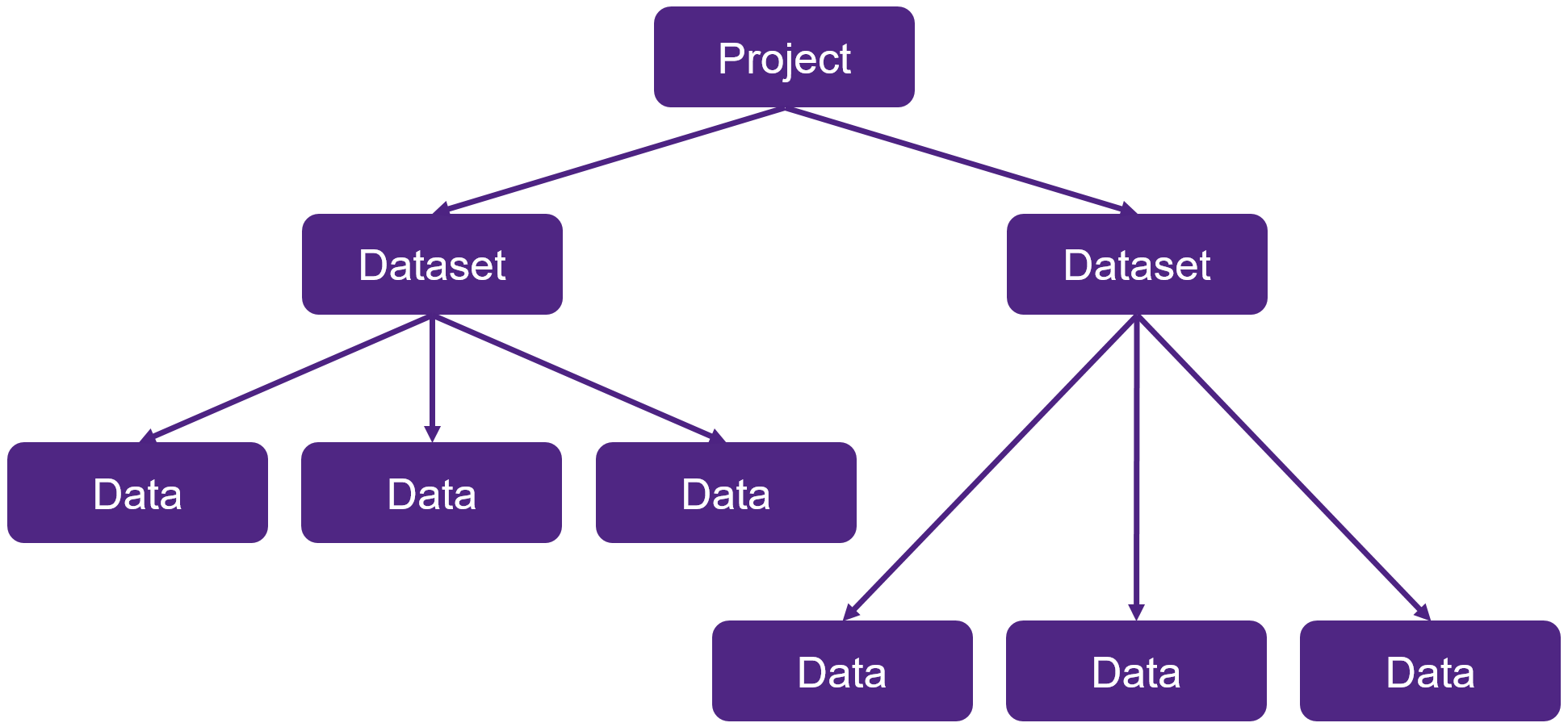
Figure 1. Organization of Project, Dataset, and Data objects in SWB Python database for TCAD to SPICE flow. (Click image of full-size view.)
The top-level object, a project, represents a single node in a Sentaurus Workbench project. A project for the current node is created automatically whenever gpythonsh is run from Sentaurus Workbench, and a Python representation of this is passed automatically to the gpythonsh scripting environment as the node_prj object.
The Dataset object represents a single invocation of a tool wrapper inside a gpythonsh script, for example, Garand VE, Mystic, or RandomSpice. Again, the dataset is created automatically by gpythonsh and then is passed to the application so that it knows where to store the data it generates.
The Data object represents a single "thing" generated by a backend simulation tool. This contains data generated by the tool and can include I–V curves, C–V curves, compact model parameters, statistical distributions, and so on. For tools that do not currently have a direct link to the SWB Python database, Data objects can be constructed from output files and stored in the database by uploading them using gpythonsh in the script.
Each instance of these objects also stores metadata associated with the current context in which gpythonsh is being executed for a TCAD to SPICE flow. For example, a Project object stores the current Sentaurus Workbench parameters and variables. This provides a powerful mechanism for navigating both horizontally and vertically in a Sentaurus Workbench project, and this is demonstrated later.
2.2.1 Project Objects
These objects have the following attributes:
- name: Label for the object, which is typically the Sentaurus Workbench node number
- metadata: A Python dictionary that contains metadata about the corresponding node
- swbparams: A shortcut to access Project.metadata["swb"]
- datasets: Provides a list of all child Dataset objects
2.2.2 Dataset Objects
These objects have the following attributes:
- name: Label used to provide a reference for the dataset
- metadata: A Python dictionary that contains metadata about the tool invocation
- parent: This links Dataset objects to the Project object (that is, the Sentaurus Workbench node) with which the tool invocations are associated
- previous: This links tool invocations within a single node (only Mystic uses this functionality)
- data: Provides a list of all child Data objects
2.2.3 Data Objects
These objects have the following attributes:
- data: Stores the simulation data itself
- metadata: A Python dictionary that contains metadata about the simulation, such as bias, temperature, and geometry
- parent: This links to the Dataset object to which the current Data object belongs
2.3 Database Interaction
In general, the requirement for user interaction with the database should be minimal. The database exists to provide data integrity throughout a tool flow without adding a significant amount of extra complexity.
In the gpythonsh scripting environment for TCAD to SPICE flows, there are different access points to the database: the dbi object and the Data class. For detailed descriptions, see the API documentation.
2.3.1 The dbi Object
The dbi object provides a comprehensive API to the SWB Python database that can be used to create, retrieve, and delete any database objects already mentioned, at any point in the TCAD to SPICE tool flow. As previously described, gpythonsh creates automatically the project and dataset structure. However, it might sometimes be necessary to create datasets manually or to retrieve objects from the database to manipulate or attach extra attributes. For each of these database objects, dbi has a create (create_dataset), retrieve (get_dataset), and delete (del_dataset) method.
2.3.2 The Data Class
Taking raw simulation data and converting it into a compatible format to save in the database can be a complex procedure. The Data class provides a Python representation of simulation data within the scripting environment that provides a straightforward interface between CSV and PLT files, and the database. It is essentially a more structured and easier to use alternative to the create_dataset and get_dataset methods of the dbi object that also provide links to external file formats. Figure 2 shows how the Data class can be used to upload a Sentaurus Device PLT file.
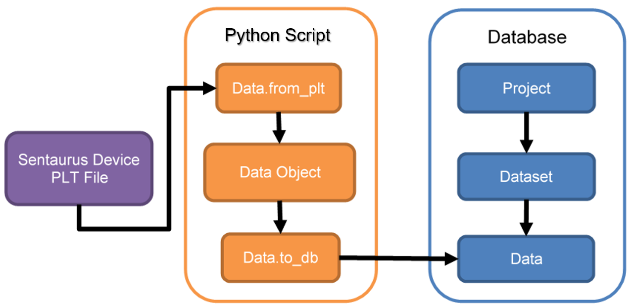
Figure 2. Using the Data class to go from a PLT file to a Data object in the database. (Click image of full-size view.)
In the gpythonsh environment for TCAD to SPICE flows, Data objects have a powerful API that can be used for numerous data manipulation operations, such as scaling, resampling, and figure of merit calculations on I–V curves.
2.4 Examples
For usage examples of the Data class, see Section 2.4.2 Uploading Data and Section 2.4.3 Retrieving Data.
This section describes some common database interactions in a TCAD to SPICE flow.
2.4.1 Attaching and Propagating Project Metadata
gpythonsh automatically creates a project for every submitted TCAD to SPICE node in a Sentaurus Workbench input file. To construct a representation of the input file in the database that can be queried effectively, it is important to attach relevant metadata to the automatically created project (node_prj) in the Python script. On creation, a dictionary representation of the Sentaurus Workbench parameters in the current row of the input file is attached to the project, which can be accessed as follows:
swb_params = node_prj.metadata["swb"]
Extra fields can be added as keyword–value pairs, where the value can be any valid Python object to the Project metadata using the add_metadata method of the node_prj object as shown here:
# Get the DoE coordinate of this point
doe = {"@axis1@": @lgate@,
       "@axis2@": @hfin@,
       "@axis3@": @tfin@,
       "@axis4@": @afin@,
       "@axis5@": @tspacer@ }

# Check whether you are at a midpoint
if (doe["@axis1@"] == @axis1_midpoint@) and \
    (doe["@axis2@"] == @axis2_midpoint@) and \
    (doe["@axis3@"] == @axis3_midpoint@) and \
    (doe["@axis4@"] == @axis4_midpoint@) and \
    (doe["@axis5@"] == @axis5_midpoint@):
    midpoint = True
    print("DOE: midpoint True")
else:
    midpoint = False
    print("DOE: midpoint False")

# Update project metadata
node_prj.add_metadata(doe=doe, midpoint=midpoint)
In this example, from the UploadData tool instance, you are adding the design-of-experiments (DoE) coordinates from an example Sentaurus Workbench input file to the project, along with a flag indicating whether the current node is at a DoE midpoint.
You might also want to propagate this metadata downstream in a tool flow to subsequent tool instances without explicitly declaring it every time. This can be done using the copy_metadata method as shown here:
# Update project metadata
node_prj.copy_metadata("@node|UploadData@")
The name of the project from which metadata will be copied is passed to the method, which is the UploadData node number in this case. Extra keyword arguments can also be added to overwrite metadata fields in the copied dictionary or to attach new fields that do not already exist.
As well as using these methods, attributes of database objects in the environment can be manipulated directly as follows:
node_prj.metadata["midpoint"] = True
node_prj.save()
In this case, the object must be explicitly saved to the database to ensure the new information is retained.
2.4.2 Uploading Data
The tools in the TCAD to SPICE flow that are tightly integrated with gpythonsh, such as Garand VE and Mystic, maintain their own backend connections to the SWB Python database, allowing them to upload simulation data directly to the gpythonsh datasets.
For tools without a direct database connection, gpythonsh must be used to gather simulation results, to attach relevant metadata, and to upload data to the database.
The following example demonstrates how to upload Sentaurus Device PLT data to the SWB Python database using the from_plt method of the Data class:
ds = dbi.create_dataset(node_prj, "ivs", clean=True)

metadata={"temperature": @temp@,
          "instances": {"l": @lgate@}}

upload_data_iv = ["@ppwd@/IdVg_0_n@pnode|IdVg@_des.plt",
                  "@ppwd@/IdVg_1_n@pnode|IdVg@_des.plt",
                  "@ppwd@/IdVd_0_n@pnode|IdVd@_des.plt",
                  "@ppwd@/IdVd_1_n@pnode|IdVd@_des.plt",
                  "@ppwd@/IdVd_2_n@pnode|IdVd@_des.plt"]

Data.from_plt(upload_data_iv,
              metadata=dict(metadata, nodes=["@drain_con@", "@gate_con@",
                                             "@source_con@", "@bulk_con@"]),
              upload_ds=ds)
When not calling a tool directly through gpythonsh, the dataset to be utilized must be created explicitly by using dbi.create_dataset before data can be stored in the database, or uploaded to the database using dbi.create_dataset.
The PLT file is parsed using the from_plt method of the data container and is uploaded to the newly created dataset ivs, using the upload_ds argument. The metadata attached to the Data object is in the form of a Python dictionary. The keywords and values are completely arbitrary. However, depending on what the data is intended to be used for, the keywords must match up with the expectations of later tools in the flow.
| Keyword | Description |
|---|---|
| temperature | Simulation temperature. |
| instances | The instances dictionary is applied to the SPICE model if the simulation data should be used as an extraction target by Mystic. Instances can be arbitrary as long as they are compatible with the SPICE model you are using. If the simulation data is not to be used as a Mystic target, the instance dictionary is not required. |
| bias | The bias dictionary identifies the voltages applied to each node during simulation. When importing from a PLT file, these values are extracted automatically from the file. The following terminal names are arbitrary but must match the supplied nodes list:
|
| nodes | List of terminal names of the device being simulated. |
Creating a unique set of metadata for each Data object can help with querying data from the database in later stages.
Click to view the UploadData Python file UploadData_eng.py.
2.4.3 Retrieving Data
Data uploaded to the SWB Python database can be retrieved at any stage in a gpythonsh workflow by using the from_db method of the Data class as shown here:
# Load simple Id-Vg data from the UploadData node
idvg = Data.from_db(project="@node|UploadData@",\
                    ivar="v@gate_con@", dvar="i@drain_con@")
The keyword arguments supplied to the from_db method are used to query the metadata stored with the data in the database. As well as the metadata dictionary attached during upload, you can query the data by type, by using the independent and dependent variable (ivar and dvar) keywords. The conventions for these keywords for different data types are shown in the following table.
| Voltage | v@node@ |
|---|---|
| Current | i@node@ |
| Capacitance | c(@node1@,@node2@) |
Hierarchical entries in the metadata dictionary such as the instances and bias fields can be matched using the double underscore syntax shown above. The example above shows low-drain and high-drain Id–Vg data being retrieved into separate Data objects from the ivs dataset created during upload.
2.4.4 Example Output
The ShowRowData tool instance is set up to showcase the database contents for a single row of data, created in the UploadData tool instance. First, you look at the metadata attached to the UploadData database node using the following commands:
UploadData_prj	= dbi.get_project("@node|UploadData@")

print("*"*32)
print(f"Upload data DB name: {UploadData_prj.name}")
print("*"*32)
print(f"Upload data metadata: {UploadData_prj.metadata}")
The print returns from these commands are shown next. You can see the database location is named after the node in the Sentaurus Workbench input file (3086). The output shows all the top-level metadata and the swb metadata that contains all of the Sentaurus Workbench parameters and variables.
Upload data DB name: 3086
Upload data metadata: {'owner': 'admin', 'members': '', 'sge_project': None,
'swb': {'Type': 'pMOS', 'sOri': 100, 'cDir': 110, 'L': 0.025, 'H': 0.04,
'W': 0.008, 'a_fin': 88, 'tt': 1, 't_spacer': 0.008, 'Fin_HM_Patterning': 1,
'HKMG': 1, 'DeviceMesh': 3, 'ElContacts': 1, 'Strain_Impact': 1, 'rcx': 0,
'Vdd_Lin': -0.05, 'Vdd': -0.8, 'WF': 4.882, 'Vgg': -0.8, 'Vgmin': -0.4,
'NVg': 3, 'axis1': 'l', 'axis1_midpoint': 2.5e-08, 'axis2': 'hfin',
'axis2_midpoint': 4e-08, 'axis3': 'wfin', 'axis3_midpoint': 8e-09,
'axis4': 'afin', 'axis4_midpoint': 88, 'axis5': 'tspacer',
'axis5_midpoint': 8e-09, 'workfn': 4.882, 'drain_con': 'drain',
'gate_con': 'gate', 'source_con': 'source', 'bulk_con': 'substrate',
'acdrain_con': 'drain', 'acgate_con': 'gate', 'acsource_con': 'source',
'acbulk_con': 'substrate', 'Vdd_nom': -0.8, 'Vdd_lin': -0.05, 'temp': 300,
'lgate': 2.5e-08, 'hfin': 4e-08, 'tfin': 8e-09, 'afin': 88, 'tspacer': 8e-09,
'rsc': 0, 'rdc': 0, 'tool_label': 'UploadData', 'tool_name': 'UploadData'},
'doe': {'l': 2.5e-08, 'hfin': 4e-08, 'wfin': 8e-09, 'afin': 88,
'tspacer': 8e-09}, 'midpoint': True}
Finally, the uploaded data can be extracted by referencing the UploadData node. In the following code snippet, all Id–Vg data is loaded from a single database location:
idvg = Data.from_db(project="@node|UploadData@",\
                    ivar="v@gate_con@", dvar="i@drain_con@")
The printed data will include two Id–Vg curves at two different drain biases. The bias information can be seen in the bias section of each data object.
Instead of using node numbers, you can also extract data based on Sentaurus Workbench level parameters. In the following example, nodes with Type=nMOS and W=0.008 are identified first, and then Id–Vd data is extracted where the gate bias is 0.6 V:
projects   = dbi.get_project(swb__Type="nMOS", swb__W=0.008)
projects   = [p.name for p in projects]
idvd_vg0p6 = Data.from_db(project=projects, ivar="v@drain_con@",\
                          dvar="i@drain_con@", bias={f"@gate_con@":0.6})
The return value of this query is a collection of seven Id–Vd curves from the splits highlighted in Figure 3.
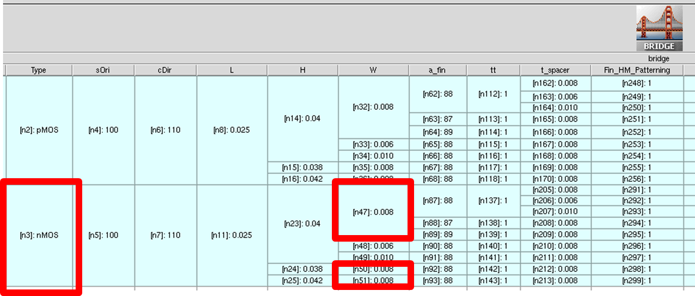
Figure 3. Highlighting the experiments selected by the database query in the previous example. (Click image for full-size view.)
Click to view the ShowRowData Python file ShowRowData_eng.py.
Copyright © 2022 Synopsys, Inc. All rights reserved.