Sentaurus Workbench
10. Optimization Framework

10.1 Getting Started
10.2 Basic Optimization
10.3 Worked Example: Trench Gate NMOS On-Resistance Optimization

Objectives

• To introduce the Sentaurus Workbench Optimization Framework.
• To demonstrate how to use the different functionalities of the Optimization Framework.

10.1 Getting Started

The Optimization Framework is a tool designed to extract efficiently general information about TCAD simulations. For example, it can be used to determine a parameter set that satisfies given design specifications or to analyze how parameter variations affect device behavior.

The Optimization Framework can be used for a wide range of purposes. It provides the following functionality:

• Optimization allows you to find an optimal parameter set for given target specifications. Multiple optimization targets can be combined, with weights specifying their relative importance. Several algorithms are available to solve optimization problems.
• Screening analysis illustrates the impact of different parameters on the simulation responses, helping you to determine the most relevant ones.
• Sensitivity analysis determines how small changes to a given parameter affect simulation responses.
• Response surface modeling fits predetermined models to data and can be used to better understand trends for interpolation, for approximating quantities of interest, and so on.

The Optimization Framework provides a Python environment that allows you to define and use custom algorithms that address specific tasks. The components of the Optimization Framework can be combined to develop an optimization strategy. For example, a screening analysis can be combined with an optimization: through the screening analysis, the important target parameters are found, and then only these are optimized.

The Optimization Framework interacts with batch tools of Sentaurus Workbench for setting up and running simulations (Sentaurus Workbench experiments).

This section covers the following topics:

• Section 10.1.1 Accessing the Optimization Framework
• Section 10.1.2 Optimization Framework Input File
• Section 10.1.3 Running an Optimization
• Section 10.1.4 Restarting an Optimization
• Section 10.1.5 Resetting the Project
• Section 10.1.6 Optimization Framework Output Log

10.1.1 Accessing the Optimization Framework

Before accessing the Optimization Framework, you must start Sentaurus Workbench in advanced mode:

swb -a &

The Optimization menu appears in the menu bar (see Figure 1).

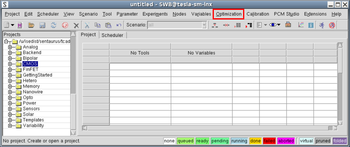
Figure 1. Main window of Sentaurus Workbench in advanced mode with Optimization menu highlighted. (Click image for full-size view.)

10.1.2 Optimization Framework Input File

The Optimization Framework input file, genopt.py, can be accessed through the menu bar of Sentaurus Workbench by choosing Optimization > Edit Python Input (see Figure 2).

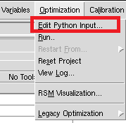
Figure 2. Optimization menu in Sentaurus Workbench.

The input file for optimization projects genopt.py is usually composed of four sections: definition of optimization parameters, definition of optimization targets and constraints, the strategy to optimize the targets and, optionally, postprocessing of the results.

10.1.3 Running an Optimization

After the optimization is set up, you can run the Optimization Framework. To run the Optimization Framework from the graphical user interface of Sentaurus Workbench, choose Optimization > Run (see Figure 2).

Alternatively, on the command line, enter:

genopt [options] [project_dir]

where [project_dir] is the path to the Sentaurus Workbench project to be executed. The Optimization Framework (genopt) will use the Python script genopt.py in the [project_dir] directory as the input file.

See the Sentaurus™ Workbench Optimization Framework User Guide for available command-line options.

10.1.4 Restarting an Optimization

Sometimes, it is necessary to restart an optimization from a previously executed optimization project. This might be because of a failure in the previous executions or because you want to change the input file while reusing all the simulations already done.

The Optimization Framework uses scenarios to define conditions from which the project can be restarted. The scenarios that can be used for restarting are initial and restart_* (for example, restart_1 or restart_2). The restart_* scenarios are created automatically with the optimal parameter values from each stage.

To restart the Optimization Framework from the graphical user interface of Sentaurus Workbench, choose Optimization > Restart From > <scenario> (see Figure 3). The Restart From command is unavailable unless a valid restarting scenario is present in the project.

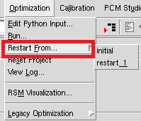
Figure 3. Menu showing command for restarting scenario.

If restarting from initial without changes to the input file, then the same optimization will be executed and all previously finished experiments reused. This is the usual required behavior when the optimization fails due to external causes (for example, network failure in the compute farm). The only exception is when a random seed selection for the random number gnerator is present in the input file:

np.random.seed()

In this case, the new optimization will diverge from the previous one after a new random number is used.

When using one of the restart_* scenarios, it will be treated as the initial scenario for the run. For example, when using the command:

optimizer.set_from_swb(params)

the parameter values will be set to the values in that scenario. As before, any experiment already executed will be reused.

10.1.5 Resetting the Project

To remove all experiments generated by the Optimization Framework, choose Optimization > Reset Project (see Figure 2). This command will keep only the experiments belonging to the scenario initial and will delete all other experiments and their outputs. The nodes belonging to the scenario initial will not be cleaned up.

10.1.6 Optimization Framework Output Log

After starting the execution of the Optimization Framework, a dialog box with the output log opens. After closing the dialog box, you can reopen it by choosing Optimization > View Log (see Figure 2).

Using the default verbosity settings, the output log shows information about the executed experiments that is useful to track the progress of the optimization.

Figure 4 shows a typical section of the output log. Each call to optimizer methods, such as optimize(), search(), and sensitivity_analysis(), is called a stage, and a header is printed at the beginning of its execution (see green box in Figure 4).

After an experiment is finished, the evaluation number is printed (this is reset to 1 at the beginning of each stage; see blue box in Figure 4) followed by the parameter values, the output values, and the total error (see red box in Figure 4).

The output values include the Sentaurus Workbench experiment from which they were extracted (the number corresponds to the last node number of the experiment), the target that was set for it, and the error contribution.

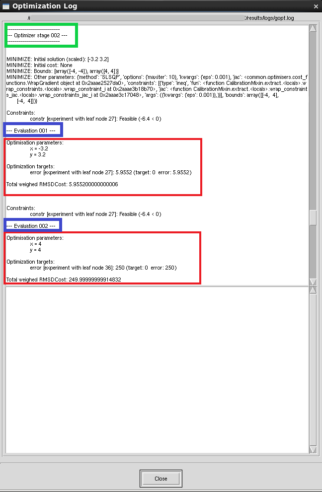
Figure 4. Output log of Optimization Framework. (Click image for full-size view.)

10.2 Basic Optimization

This section explains how to set up an optimization project and its main components, through a simple example using an analytic function.

The project used here can be found in the Applications_Library directory. Figure 5 shows the original state of the project.

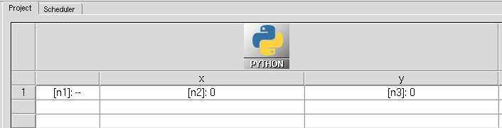
Figure 5. Sentaurus Workbench project before running the Optimization Framework. (Click image for full-size view.)

In general, an optimization project can include any TCAD process and device simulations as Sentaurus Workbench usually does. In this simple example, it consists of a single Python tool with the following input:

x = @x@
y = @y@

value = (x**2+y-11)**2 + (x+y**2-7)**2
constraint = x - y

print(f"DOE: error {value}")
print(f"DOE: constr {constraint}")

The input to the tool are the two Sentaurus Workbench parameters x and y, referenced in the first two lines using the preprocessor commands @x@ and @y@. The Optimization Framework relies on Sentaurus Workbench parameters to define the input space, so the tools using parameters that need to be optimized have to take their values using preprocessor directives as in this example.

As the outputs, the tool calculates the value of an analytic function (value) and the value of a function that will be used to define the constraint x < y (constr), see Figure 6. In order for the Optimization Framework to be able to use these values, they must be written as Sentaurus Workbench variables, which is achieved using the print commands.

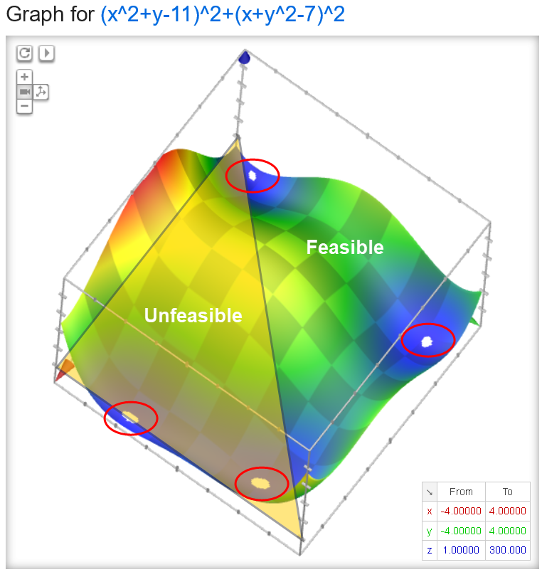
Figure 6. Test function used for optimization. (Click image for full-size view.)

The input file (choose Optimization > Edit Python Input) defines an optimization strategy possibly composed of several tasks. This file is a Python script with some additional classes and objects injected into the environment related to the Optimization Framework, including the following:

• optimizer is the main object of the Optimization Framework. Internally, it drives the optimization process and manages the Sentaurus Workbench project. Optimization tasks are invoked using methods of this object.
• OptParam and TOptParam are classes that represent optimization parameters. They manage parameter value, bounds, and transforms (TOptParam).
• OptTarget is a class that represents targets for the optimization process. In general, it needs the response (simulation output, possibly postprocessed) and a target value for the simulation output. You can specify additional properties such as a weight.

10.2.1 Optimization Parameters

The first part of the input file of the project is the definition of the optimization parameters:

x = TOptParam('x', 0, -4, 4)
y = TOptParam('y', 0, -4, 4)
params = [x, y]

optimizer.set_from_swb(params)

The first two lines define a parameter using the TOptParam class. The first argument ('x' and 'y') is the name of the Sentaurus Workbench parameter to be optimized, the second argument is the initial value, followed by the lower and upper bounds for the parameter. The parameters are grouped into the list params for convenience for later use. Finally, using the set_from_swb method of the optimizer object sets the value of the parameters to the value currently assigned in the project. In this example, the values are the same but, in general, this command will maintain consistency between the input file and the project.

10.2.2 Optimization Targets

Optimization targets are used to define the quantities that need to be optimized. Together with the constraints, they define the output space of the optimization problem.

In the Optimization Framework, targets and constraints are defined based on Sentaurus Workbench project variables, which, in general, are written by the simulation tools or postprocessing stages. For this example, the target definition is:

# Define optimization targets
t1 = OptTarget("error", value=0, scale=1)
targets = [t1]

These commands define an optimization target that will try to match the output variable errors to the target value of 0.

As shown before, the output of this example has four minima. Constraints can be used when you know that the optimal solution should verify some additional condition. In this case, you add a constraint to retrieve solutions with x < y:

# Define constraints (x-y<0)
c1 = OptConstraint("constr", lt=0)
constraints = [c1]

where lt means less than. As previously described, the output variable constr contains the value of x-y, so the applied constraint is constr < 0.

10.2.3 Optimization Strategy

After the parameters and the targets have been defined, the third and central part of the optimization is to define the strategy, that is, how to combine parameters and targets to reach the optimal solution.

The example has two parts: one global search and one local minimization. Since the function you want to minimize is not convex, you will try to find a good starting point before using a local minimization algorithm to find the minimum.

10.2.3.1 Parameter Space Search

The call to optimizer.search executes the problem in a series of points and returns the best value. For example:

# Parameter search - Grid
opt_params = optimizer.search(params, targets + constraints,
	method="grid", options={"Ns": 5}
)

In this example, method="grid" indicates that the points to execute define a grid in the input space defined by params, and the option "Ns": 5 means that this should be a 5x5 grid. For each of the 25 experiments, the target and constraint will be evaluated, and the call will return the parameter values that produce the lowest target while satisfying the constraint.

10.2.3.2 Local Optimization

The example uses a local minimizer to refine the value found by the search. The options for local minimization are set through the backend, which can be accessed using optimizer.backend. For example:

# Local minimization
optimizer.backend.set_method("minimize")
optimizer.backend.set_optimization_parameters(jacobian_options={"eps": 1e-3},
                                              method="SLSQP",
                                              options={"maxiter": 10})

In this example, you chose the backend minimize, which gives access to the general minimization algorithms. The algorithm chosen was SLSQP, which is a gradient-based optimization algorithm that admits general nonlinear constraints. Finally, to limit the number of experiments created, the option maxiter is set to 10.

After the options for the backend have been set, you can run the local minimization, such as:

opt_params = optimizer.optimize(params, targets + constraints)

As before, the call to optimizer.optimize takes the parameters, targets, and constraints.

10.2.4 After the Optimization

The Sentaurus Workbench project is updated and refreshed as the optimization progresses, so all intermediate results produced by the simulation tools are available. Figure 7 shows the project after the optimization is complete.

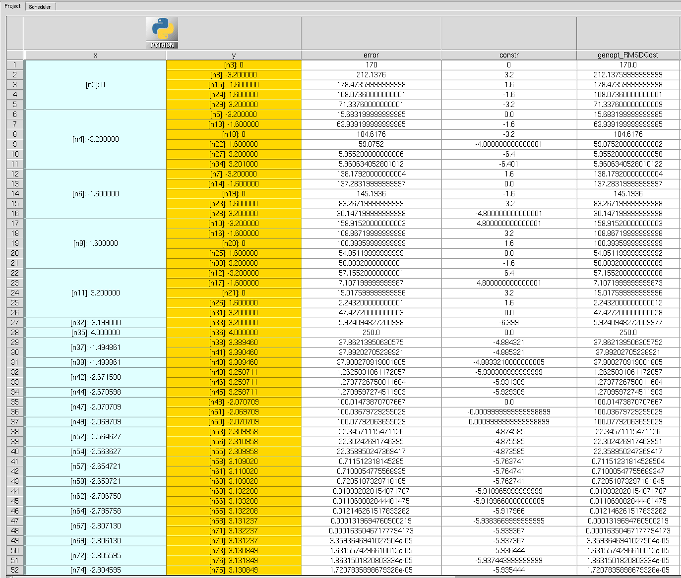
Figure 7. Sentaurus Workbench project after running the Optimization Framework. (Click image for full-size view.)

To simplify the visualization of the optimizer project, all experiments are added to additional scenarios. Figure 8 shows the scenario list after the optimization.

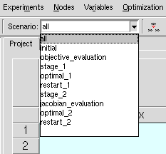
Figure 8. Scenarios after running the Optimization Framework.

The created scenarios contain the following experiments:

• objective_evaluation: Experiments in the main optimization trajectory.
• jacobian_evaluation: Experiments used to evaluate the numeric approximation to the Jacobian used to drive the (gradient-based) optimizations.
• initial contains the experiments of the initial project.
• optimal_1, optimal_2 contain the experiments executed using the optimal set of parameters after the call to optimizer.search() and optimizer.optimize(), respectively.
• restart_1, restart_2 contain a copy of the scenario initial in which the optimization parameters have been replaced by the optimal ones after the call to optimizer.search() and optimizer.optimize(), respectively.
• stage_1 and stage_2 contain all experiments (excluding Jacobian evaluations) executed in the call to optimizer.search() and optimizer.optimize(), respectively.

10.2.4.1 Output Data

In addition to the data generated by the experiments, some data generated by the Optimization Framework is available in the genopt_plots and genopt_data folders in the optimizer node folder. To access the data using the Sentaurus Workbench Node Explorer, follow the steps shown in Figure 9.

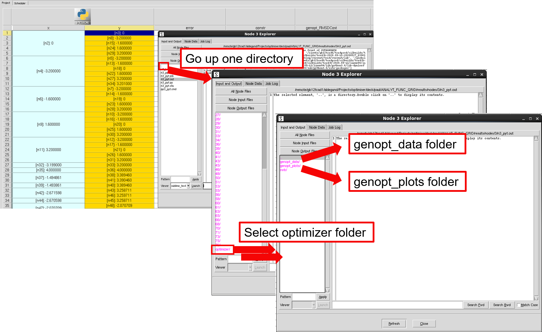
Figure 9. Path to optimizer output folders. (Click image for full-size view.)

The genopt_data folder contains a CSV file for each stage of the optimization, which lists the ouputs, output errors (distance to target), and the total error, as shown in Figure 10. Note that ouput columns are in brackets. You might need to remove them before using this file directly in a plotting application.

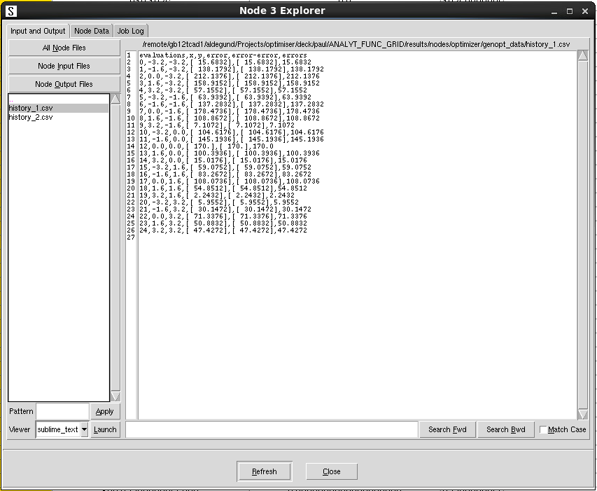
Figure 10. The genopt_data folder after running the Optimization Framework. (Click image for full-size view.)

The genopt_plots folder contains any figure created by the Optimization Framework, as shown in Figure 11. In this example, the convergence plot was created by the call to optimizer.optimize, but it also includes the data from the call to optimizer.search.

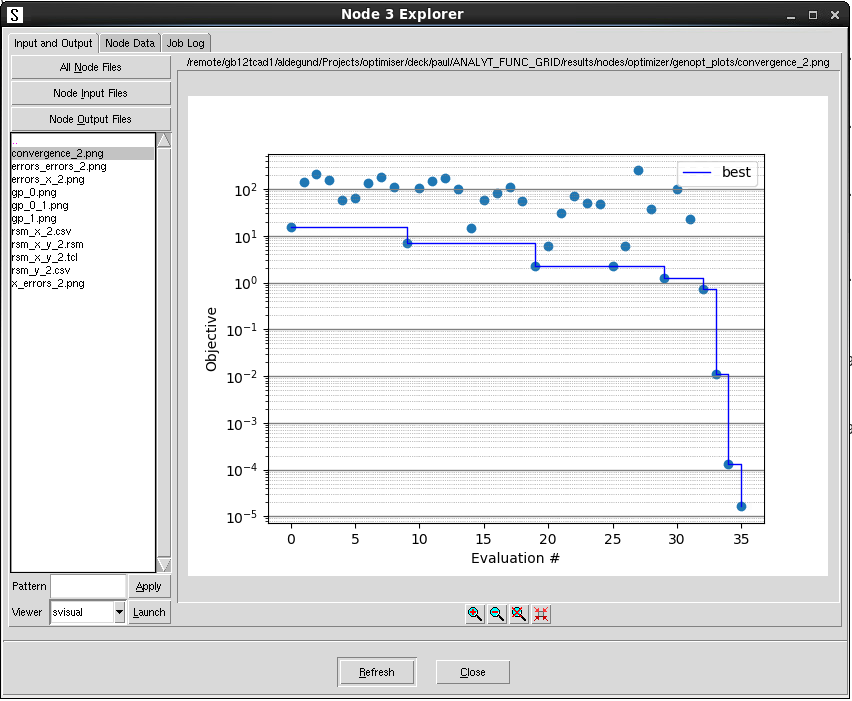
Figure 11. The genopt_plots folder after running the Optimization Framework. (Click image for full-size view.)

The plots gp_*.png and rsm_* contain 1D cutlines and 2D cutplanes of a response surface model (RSM) fitted to the total error in the call to optimizer.search. Figure 12 shows the 2D RSM contour levels, where black dots are the locations of the simulations, and the background crosses represent the uncertainty in the RSM, with blue shades indicating lower uncertainty and red shades indicating higher uncertainty.

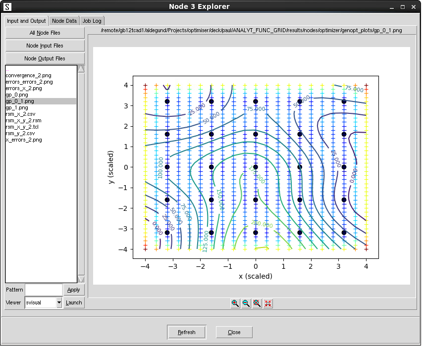
Figure 12. Two-dimensional RSM file. (Click image for full-size view.)

Figure 13 shows one of the 1D cutlines, which are taken at the best point found. In this plot, circles are again simulation data. Since the data is 2D, not all points are at the same distance of the cutline. The distance is represented by the background color of the circle: the darker the color, the closer to the cutline. This plot shows the characteristic double well as seen before in the plot of the function in Figure 6. The blue line corresponds to the average prediction of the RSM and the thin red lines show ± one standard deviation around the mean of the prediction.

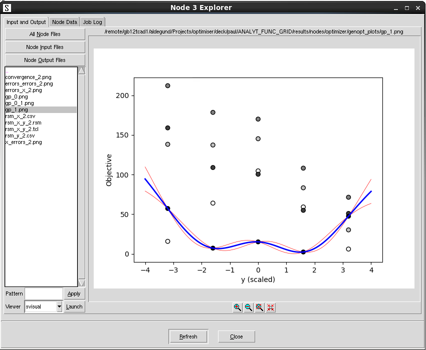
Figure 13. One-dimensional cutline of the RSM. (Click image for full-size view.)

The files rsm_*.tcl and rsm_*.csv contain the RSM data in a format that can be opened in Sentaurus Visual, as shown in Figure 14.

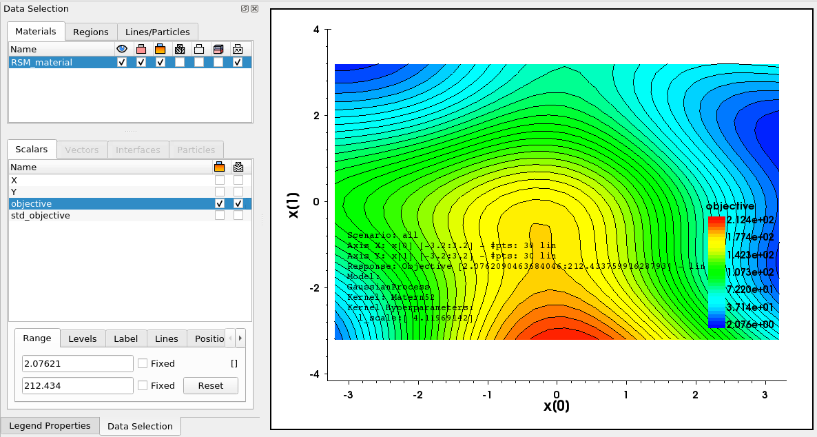
Figure 14. RSM file opened with Sentaurus Visual. (Click image for full-size view.)

10.3 Worked Example: Trench Gate NMOS On-Resistance Optimization

This section guides you through the optimization of process conditions for a trench gate NMOS device to achieve a low on-resistance, while ensuring that the breakdown voltage does not drop below a given value.

10.3.1 Trench Gate NMOS Structure and Project Organization

The example used here is a trench gate NMOS device. Its structure is shown in Figure 15.

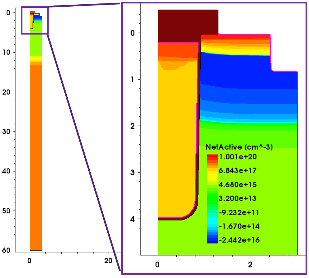
Figure 15. Structure of the trench gate NMOS example. (Click image for full-size view.)

A TCAD input file is set up to use Sentaurus Device to simulate the I_d–V_g, I_d–V_g, and breakdown characteristics of this trench gate NMOS device, as shown in Figure 16. From the I–V results, the threshold voltage (Vth), on-resistance (Ron), and breakdown voltage (BV) can be extracted (using Sentaurus Visual here).

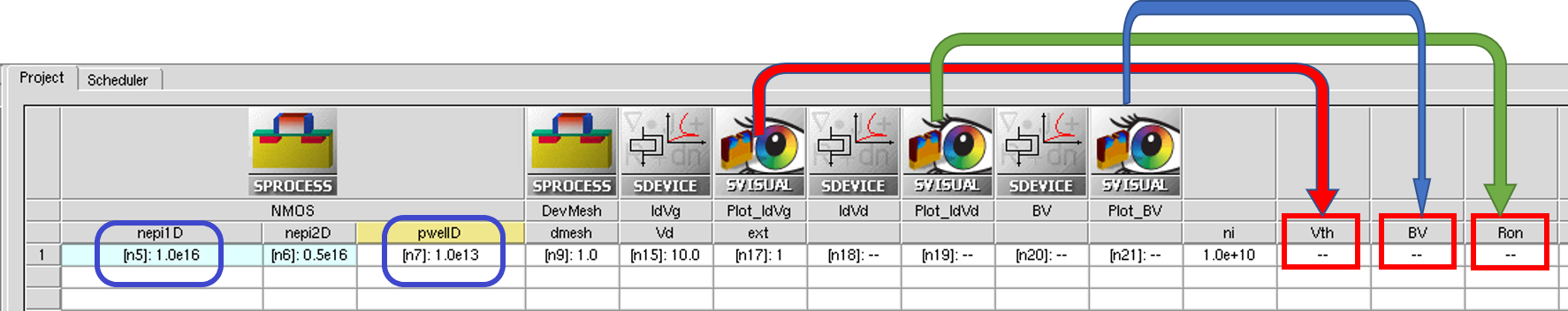
Figure 16. TCAD input file for trench gate NMOS example. (Click image for full-size view.)

Ron and BV will be affected by the process parameters, for example, nepi1D and pwellD. The example illustrates how to use the Optimization Framework to optimize process parameters to output a device with minimal on-resistance under the condition that the breakdown voltage is larger than 80 V.

For an optimization project, the parameters that need to change must be exposed as Sentaurus Workbench parameters, and the outputs used to calculate the target values must be exposed as Sentaurus Workbench variables.

10.3.2 Define Optimization Parameters and Targets

As in the previous example, the beginning of the input file includes the definition of the optimization parameters and targets.

# Define optimization parameters. Names must be Sentaurus Workbench parameters.
a = TOptParam('nepi1D', 1.0e16, 1.0e15, 2.0e16, Log10)
b = TOptParam('pwellD', 1.0e13, 1.0e12, 1.0e14, Log10)
params = [a, b]

This defines two optimization parameters corresponding to the Sentaurus Workbench parameters nepi1D and pwellD. In this case, a logarithmic transform is applied to these parameters, so the optimization internally is performed for log10(nepi1D) and log10(pwellD). This is especially useful for parameters spanning orders or magnitude.

This problem has only one target, the on-resistance, that you want to minimize. It is defined as follows:

# Define optimization targets
t1 = OptTarget("Ron")
targets = [t1]

In addition to the target, you define a constraint on the breakdown voltage, which is written to the Sentaurus Workbench variable BV, to be greater than 80:

# Define optimization constraints
c1 = OptConstraint("BV", gt=80.0)
constraints = [c1]

10.3.3 Optimization Strategy

The optimization strategy is also defined in the input file. In this case, it consists of two parts: initial search and local minimization around the best value.

10.3.3.1 Initial Search

First, you sample the input space using a Sobol sequence:

## Parameter Search
opt_params = optimizer.search(params, targets + constraints,
	method="sobol",
    options={ "Ns": 20 }
)

This will generate a sample of 20 points distributed uniformly through the transformed input space. Using an initial search is useful to better understand the behavior of the targets and also to select a good starting point for the local minimization.

Figure 17 shows the initial sampling and an RSM fitted to the data (ignoring the constraint) to give an idea of the change of the target with the inputs.

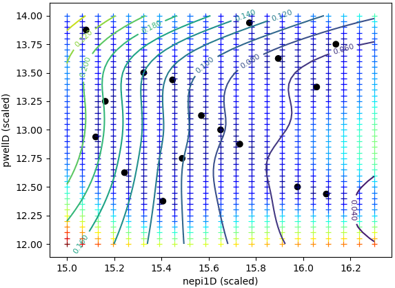
Figure 17. Initial sampling and RSM fitted to the target ignoring the constraint.

Figures 18 shows 1D cutlines along both dimensions at the optimal point. The best feasible solution is highlighted with the dashed lines. It is clear that many points for larger values of nepi1D give a lower on-resistance, but they violate the constraint set on the breakdown voltage. This can be clearly seen in Figure 19, comparing the breakdown characteristics of the search optimal and node 54, which has a lower on-resistance but violates the constraint.

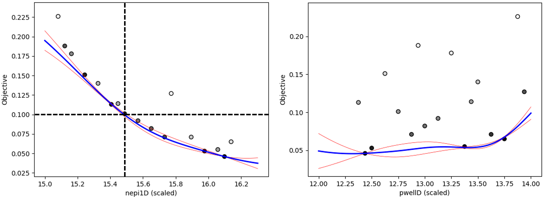
Figure 18. One-dimensional cutlines of the initial sampling and RSM fitted to the target ignoring the constraint. (Click image for full-size view.)

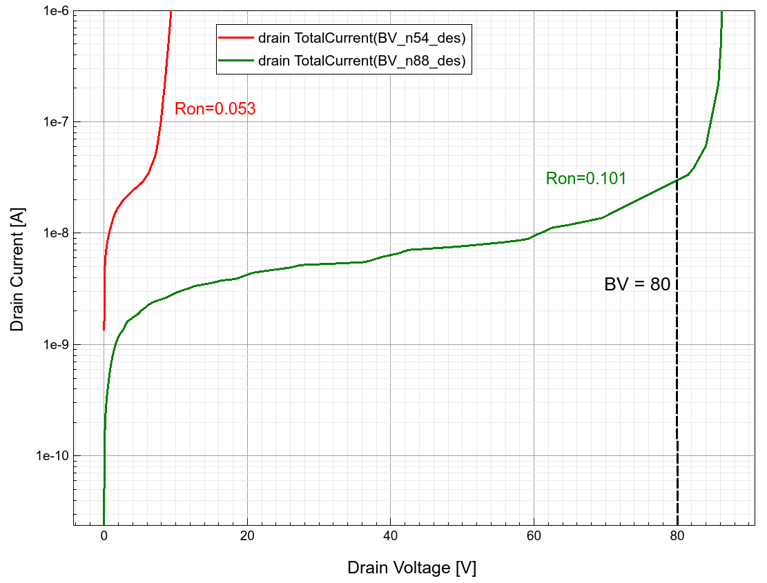
Figure 19. Breakdown voltage plots for the node with the lowest on-resistance (54) and the node with the lowest on-resistance satisfying the breakdown voltage constraint (88) during the search. (Click image for full-size view.)

10.3.3.2 Local Optimization

After the initial search, you perform a local minimization to polish the best result found in the initial search. The only gradient-based method that can take into account the constraints is SLSQP, which is available through the minimize backend:

## Local minimization
optimizer.backend.set_method("minimize")
optimizer.backend.set_optimization_parameters(
	jacobian_options={"eps": 1.e-2},
    method="SLSQP",
    options={"ftol": 1e-4, "maxiter": 10}
)

opt_params = optimizer.optimize(params, targets + constraints)

To limit the runtime, you set the maximum iterations of the algorithm to 10 and set a tolerance for the change in the target function to 1e-4.

Figure 20 shows the convergence of the local minimization after the initial search. Red boxes denote unfeasible solutions. The minimization algorithm seems to be approaching the local minimum from the unfeasible part of the space, finding a feasible local minimum after trying several better unfeasible solutions.

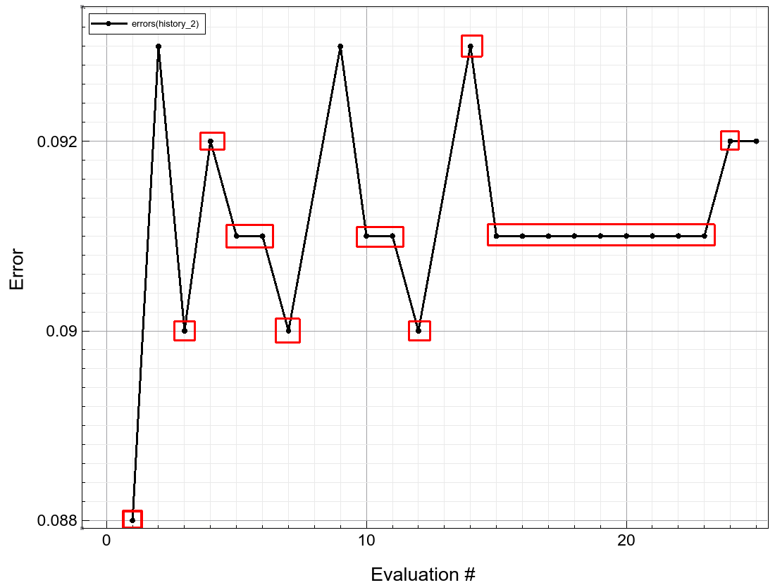
Figure 20. Convergence of the local minimization after initial search. Red boxes denote unfeasible solutions. (Click image for full-size view.)

This contrasts with the local minimization, if you ignore the constraints, which converges quickly to a local minimum as seen in Figure 21. However, this local minimum violates the required constraint with a value of BV=52 V.

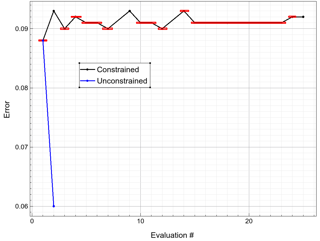
Figure 21. Convergence of the local minimization after initial search. Blue lines correspond to an unconstrained minimization. (Click image for full-size view.)

10.3.4 Optimization Results

After each optimization task (for example, search or optimize) is finished, a new scenario is created with the name prefixed by optimal_ and the task number. In this example, two optimal scenarios are created: optimal_1 and optimal_2. For example, Figure 22 shows the content of scenario optimal_1, which corresponds to the best solution found by the initial search.

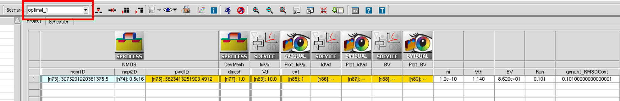
Figure 22. The optimal_1 scenario after optimization. (Click image for full-size view.)

Figures 23 and 24 show the change in I_d–V_d and breakdown curves before and after each step: initial, after the search, and after the local minimization. The final local minimization pushes the on-resistance to a minimum, while pushing the breakdown voltage to the minimal-allowed value.

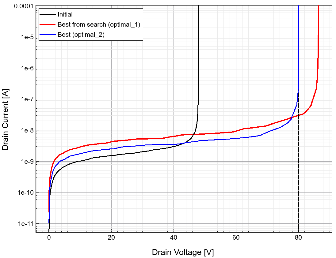
Figure 23. Breakdown curves for initial, optimal_1, and optimal_2 scenarios. (Click image for full-size view.)

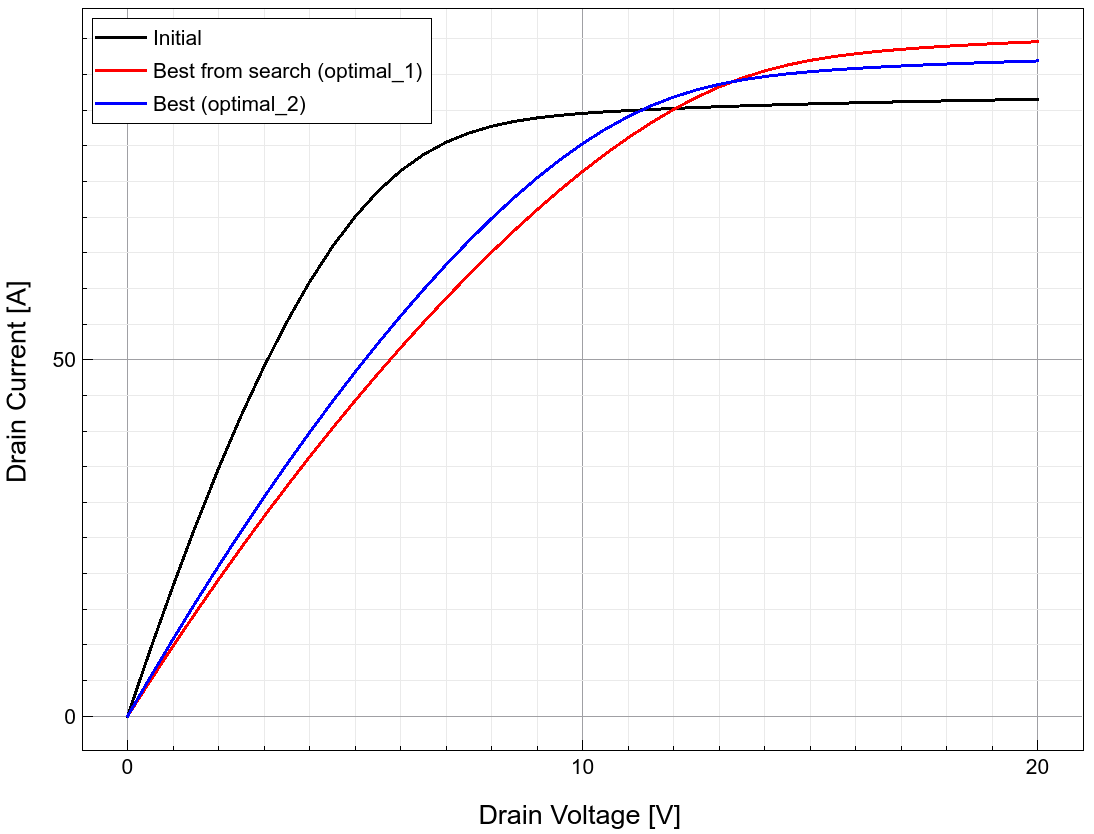
Figure 24. I_d–V_d curves for initial, optimal_1, and optimal_2 scenarios. (Click image for full-size view.)